March 19th 2020 produced an interesting news story from TASS regarding a new Konteyner 29B6 OTHR system that is to be deployed in the Kaliningrad Oblast.
Now, I still have my doubts about it being deployed here, and my first impressions were that it was just propaganda, but it still needs analysing to see what it could produce.
The article, sourcing a “Military-industrial complex”, mentions that the system is to cover the whole of Europe, including Great Britain.
This is, in itself, interesting as most of Europe is actually already covered by the system at Kovylkino. The mention of Great Britain specifically also is interesting as another Konteyner OTHR to cover this country would really only give an extra few seconds of warning that anything was coming from this direction. Moreover, I suspect that the Kovylkino system does actually cover Great Britain anyway, especially with the pulse rates of the system that I’ve analysed myself.
Looking at the image below you can see that if a system was placed at the rough centre of the Oblast, then only France, Spain and Iceland – along with GB – would be the extra countries that would be covered. The east of France is already covered as it is.
Personally, I wonder if – whilst GB might get extra coverage – the true targeting of the system would be to the North.
The Russian military have long been saying that they want to cover the Barents Sea and up to the North Pole with an early warning radar – specifically Konteyner – so this could be it.
If we adjust the predicted coverage to the North in an image then you get the following.
So, depending on the azimuths of the arrays used, we can see that GB, Iceland, East Greenland, North Sea, Norwegian Sea, Barents Sea, Norway, Sweden, Finland, Svalbard archipelago and the Noveya Zemlya archipelago (Severny Island and Yuzhny Island) could be covered by a four array system.Norway and Sweden are already partially covered by Kovylkino.
To me, this is the more likely coverage that will be created SHOULD a Konteyner system be placed in the Kaliningrad Oblast. And it is a should!
The TASS article states that multiple sites are being considered. The system at a minimum requires two sites. And the Oblast is not very big.
In all reality, the city of Kaliningrad itself is just 30 km from the Polish border. It would not take very long for a strike from a foreign land based missile site to reach a Konteyner site in the centre of the Oblast. It is because of this fact that I have my doubts about one being sited here, but who knows?
But say they do choose the Oblast for system two, where’s the likely spot?
If anything is to go by, with their previous sites, near an airfield seems to be a good choice, be it one in service, or one that could be quickly reinstated.
There’s a number of abandoned sites, including:
Chernyakhovsk at 54°36’7.12″N 21°47’29.07″E
Nivenskoye at 54°33’48.13″N 20°36’13.02″E
Marienkhof at 54°51’57.25″N 20°11’0.92″E
Chernyakhovsk has a large military presence – as does the whole of the Oblast to be honest! – and some work has been started at 54°39’1.12″N 21°48’24.77″E that I’ve been monitoring since mid 2019. Here there have been a number of small buildings about 3 metres wide since at least 2005 but I think these are something to do with oil or gas extraction – as is the new development. Moreover, the shape isn’t right for Konteyner as can be seen below.
Marienkhof (Dunayevka) is the location of a Voronezh-DM Early Warning radar that is situated to the SE of the old airfield. There is plenty of land around here for extra development. Moreover, out to the west coast is Yantarny which is home to the 841st Independent EW centre, and to the north is a SIGINT site at Pionersky that houses one of the new Sledopyt satellite signal interception systems amongst others.
Voronezh-DM Early Warning radar site near old Marienkhof airfield
Nivenskoye certainly has a lot of land available, but it is the nearest site to the Polish border and certainly not top of my list.
My favourite area would have to be near to Marienkhof due to the location of other Russian systems of this “type” – radio/radar/SIGINT based systems. The area is almost as far as you can get from any land based threats, though of course anything from the sea would not be that far.
I guess we’ll just have to wait and see what develops. One thing is for sure, the system stands out once you have an area of interest and this area is not that big to continually monitor.
For a while, sites like these in the Kaliningrad Oblast took my interest as they were developed a few years ago – this one situated at 54°28’10.14″N 21°39’4.07″E – as they looked liked potential radar or antenna sites. But it soon became obvious they were actually something to do with cattle farming
There has also been mention of another Konteyner site already in construction in the far east. At this time nothing has been found of any construction site that looks to be a Konteyner OTHR and I have my doubts about this. It was first muted in 2010, then again in 2018, and I would have expected something to be there by now.
Well, thanks to a contact on Twitter – Krakek – this has been proven not to be the case!
He was able to point me to the location of the receiver site, though it is very clear that the system has either been abandoned, or it has been postponed.
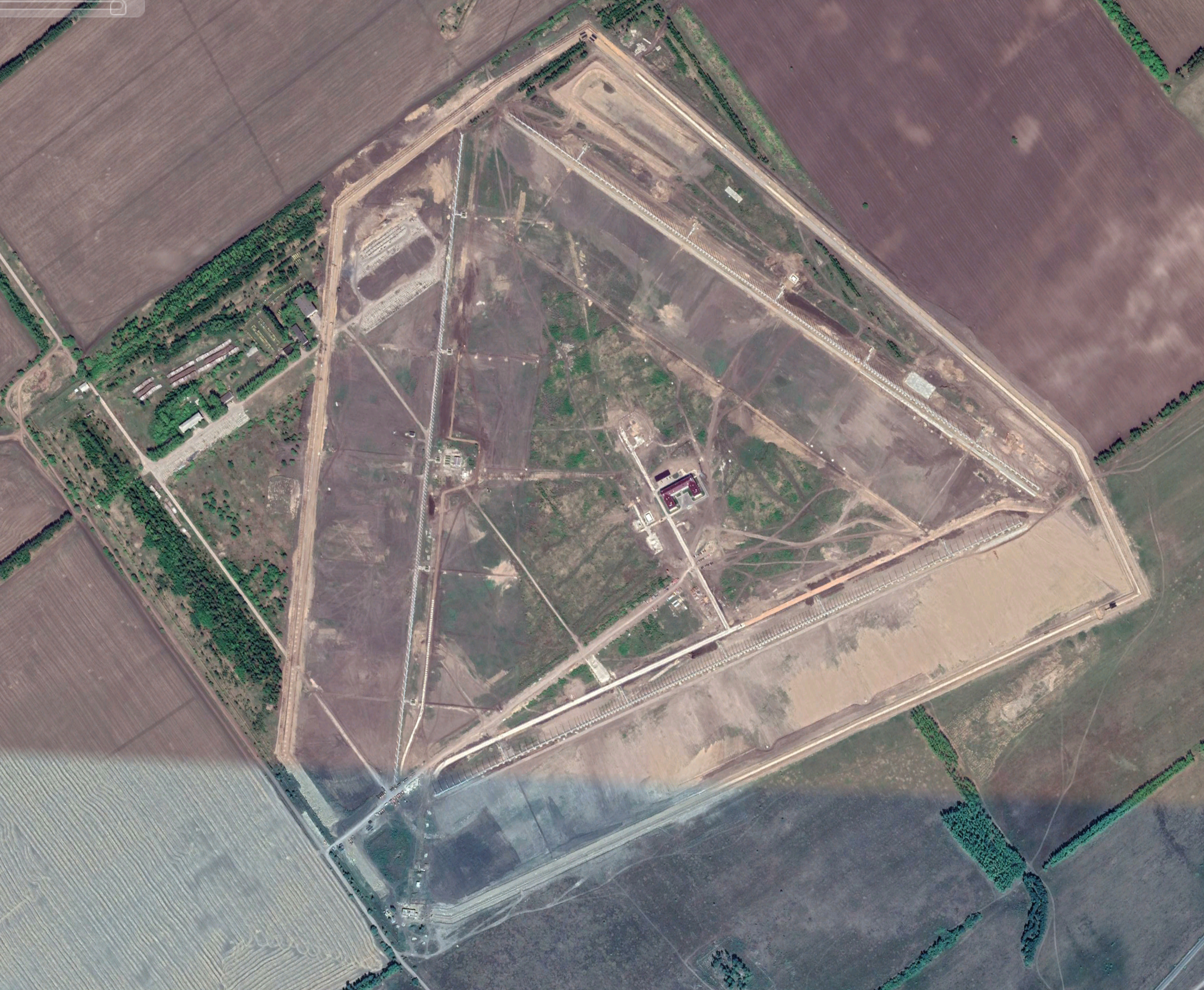
Located at 53°43’16.27″N 127° 4’29.63″E, the site appears to have been started sometime between 23rd August 2015 and 6th September 2017 according to Google Earth imagery. The site has just been cut through a forest and it appears that no antenna arrays have ever been sited there.
The latest GE imagery available, dated 7/7/19, is shown below with the site not changing since September 2017.
The site is located 9 km west of the town of Zeya. There appears to be no other real military presence, with the region being mainly involved in open pit gold mining. The large dam nearby is also a big employer – an ideal source for the large amount of electricity required to power an OTHR.
At this time I have been unable to locate any sign of the Transmitter site, though it is like looking for a needle in a haystack. I went along the same lines of the other site and looked within a nearby radius and discovered nothing of real significance.
Using the GE imagery, I’ve taken a look at the potential coverage the Far East system would provide. As there isn’t a transmitter site available, I’ve based it on a three array system, rather than the four at Kovylkino.
The image below shows the site with added arrows for the direction the antenna arrays would appear to be planned in covering. The rough bearing for each is: 077 (Green), 137 (Red) and 197 (Blue).
The Green and Blue directions are definite as you can also see the areas cut out of the trees into what would be the ground plane that is placed in front of each array. This is not visible with the Red arrow and there isn’t a second ground plane visible for an array pointing to the West. This currently points to a three array system, but should there be a fourth array, my thoughts are that it would be back to back with the Green array. My reasoning for this? The second cut through the trees that extends in front of the Red (197 degrees) proposed array and around to the rear of the Green (077 degree) is the potential extension for the ground plane.
The next image depicts the potential coverage based on the same dimensions from the Kovylino system. The quadrants are colour coded the same as the previous image. The inner ring is at approximately 900 km and shows the skip area, whilst the outer ring is at approximately 3000 km. The lines in each coloured quadrant are extend from the planned arrays to the bearings of 077, 137 and 197 degrees.
As you can see, the OTHR is perfectly placed to cover SE China, North and South Korea, Japan and anything launched from the West coast of the USA. Three of those countries have ICBM capability. Major cities and naval bases such as Vladivostok are covered, as is a lot of the sea areas to the east of Russia.
You can also see that if a fourth transmitter array was to be built and it was put back to back with the 077 (Green) system, that it would point in the direction of India and Pakistan – both countries are ICBM capable.
It will be very interesting to monitor this site, to see if any further development takes place. I wonder whether they are waiting on how well the Kovylkino site copes in a live environment before continuing with any work here.
Krakek was also able to provide me with some further data on the Konteyner system as a whole. The data, shown below with some of the information translated in a separate table, is from the procurement datasheet produced by Радиотехнические и Информационные Системы (Radio Engineering and Information Systems JSC). The paper is further sourced from Oружие Oтечества (Weapons of the Fatherland) – a fantastic site on all things Russian military. Unfortunately, I couldn’t find the direct link to the page.
This data confirms much of that already known, in particular the range (min and max) of Konteyner and the maximum number of aircraft that can be tracked simultaneously. Of note is the pulse length – 6 to 8 ms as I was able to ascertain through my analysis.
1
Multifunctional Radar Station with increased range of detection of air objects
2
Main Technical specifications
3 and 4
Wavelength Range : Decametre
5 and 6
Antenna Type : Phased Array
7
Area of Responsibility
8
Maximum Range – 2700 km
9
Minimum Range – 1000 km
10
Azimuth Width in Degrees – 60
11
Within Area of Responsibility
12
Number of continuous monitoring zones – 4
13
Range size – 450 km
14
Azimuth Width in Degrees – 15
15
Standard errors of measurement
16
Range for single target – 18 km
17
Range for single target in degrees – 2
18
Radial speed (pulse rate) – 6 to 8 milliseconds
19
Number of simultaneously tracked targets – 350
20
Service life – 15 years
21
Placement Options
22
Relocated (note – presumed mobile)
Stationary
The positional error information highlights the issues with OTHR. The plot for each track could be anything up to 18 km and/or 2 degrees out. This shows why the system can not be used for weapons targeting, and can only be used in an information or rough intercept/search area purpose for aircraft or another air defence system.
The title of the paper also alludes to the fact that Konteyner will only be used for air targets and not maritime surface targeting. This explains why there are no ship targets in the video for the Kovylkino activation.
I’d like to thank Krakek again for all the information as this has helped not only in locating the Far East site for further observations, but also for the datasheet that has proven a lot of the analysis already carried out.
I’ll be working with Jane’s, keeping a close eye on the site to catch any further work that may start here in the future.
Thanks to SDRplay, I was sent both their new RSPdx and older RSPduo SDRs at the end of January.
The main reason was to get them integrated into Procitec’s go2MONITOR and go2DECODE software, to increase the number of SDRs that the company’s products are compatible with.
This I’ve been successful in doing with the RSPdx – I’m still to unbox the RSPduo at this time of writing.
First of all though, I’ve been extremely pleased with the RSPdx in its own right. The SDRuno software works really well, is pretty easy to use – and it looks good too.
SDRuno running the RSPdx The RSPdx also works with SDRConsole
The fact that you can have up to 10 MHz of bandwidth is brilliant, and it isn’t too bad on the CPU usage either – running at around 25% with 10 MHz bandwidth on my ancient PC. Used with SDRConsole you can cover a good number of frequencies at once, and can record them if necessary. Of course, you can do this with SDRuno too, but at the moment only IQ – you can’t record individual frequencies.
Saying that, I’ve seen the SDRuno Roadmap for future releases and not only will recording of individual frequencies be possible, a more advanced scheduler is to be included. This is something I feel SDRConsole – amazing though it is – is lacking when it comes to single frequency recording. There is also the issue with SDRConsole that you are limited to recording only 6 hours worth of wav file per frequency.
Anyway, I digress. Back to the RSPdx and go2MONITOR.
To get the SDRs to work correctly with any of the go2 products means creating a configuration file and adding a ExtIO DLL file to the software. This is reasonably easy to do once you get use to it and it enables a GUI to become active so that you can control the SDR through go2MONITOR.
One interesting aspect with the RSPdx GUI is that regardless of what you enter as some of the parameters in the configuration file, the ExtIO file overrides these. Effectively, I just left some of the data as found in a basic configuration template and let the GUI do all the work for me.
So, below are some of the results with today’s first test.
First of all I went into the VHF/UHF side of things and targeted the local TETRA networks. These were found easily and after messing around with the GUI, I was able to get go2MONITOR set up to nicely find all the emissions within the 1.6 MHz bandwidth I’d chosen to use
From there, all I had to do was to select one of the found emissions and let the software do its thing.
Next I moved on to HF where there’s a plethora of data to choose from to test out the SDR. There was quite a large storm going through at the time and my Wellbrook loop and coax feed were getting a bit of a bashing with some considerable interference being produced with the really strong gusts, as can be seen below – the interference between the two HFDL bursts is one such gust.
I’ve frequently mentioned the Results Viewer that’s part of go2MONITOR and with things such as HFDL and TETRA, that process data quickly from lots of signals, this part of the software comes into its own.
The image below is two minutes of HFDL monitoring. All the red blocks is received data that scrolled through the Channel window too quickly to read live. In the viewer you can select any of the signals and you’ll be shown the message as sent. In this case, it is one sent by an Open Skies Treaty observation flight OSY11F.
By looking at the Lat/Long and comparing it to the flight history from FlightAware and its location at 1313z it ties in nicely. This flight was carried out by the German Air Force A319 1503 specially kitted out to make these flights.
go2MONITOR has a basic map function within the Result Viewer function so if there’s any Lat/Long position within any message it will plot it – as shown below for OSY11F at 1313z.
Within the General tab of Result Viewer you can get all the parameters of the signal.
One final test that I carried out was how well everything coped with a bigger bandwidth. In HF I can use up to 3 MHz of bandwidth with the licence I have – going up to 10 MHz once into VHF/UHF. In HF then, I selected 3 MHz in the GUI and then ran an emissions search.
My PC is nearing the end of its life but it coped easily with the amount of data found despite only having 4 GB of RAM with a 3.6 GHz AMD processor – a new PC is in the pipeline that is going to give me much better processing power.
Despite having 3 MHz available, not everything was identified. Most of this was at the fringes of the bandwidth, but some of the weaker signals also failed. That doesn’t mean you can’t then process them further, you can, it’s just the Emissions scan hasn’t quite been able to ID them. Saying that, the software managed to ID things within 2.2 MHz of the 3 MHz bandwidth.
I picked one of the weaker signals to see how both the RSPdx and software coped and they did very well, pretty much decoding all of the CIS-50-50 messages that were coming through on 8678 kHz.
So, overall, pretty pleased with how the RSPdx works with go2MONITOR.
Once I get a better PC I’ll be able to test at bigger bandwidths but even with 3 MHz here I was able to achieve the same, if not better, results than I have with the considerably more expensive WinRadio G31 Excalibur I have been using previously (running with the G33 hack software).
Not that I’m likely to really use go2MONITOR at big bandwidths – 1.6 MHz is probably fine for me – but for Pro’s there’s no doubt that having these “cheaper” SDRs would make absolutely no difference over using an expensive one such as those in the WinRadio range. In all honesty, I don’t think I’ll be holding on to the WinRadio for much longer – I’m more likely to get another RSPdx to cover this area of my monitoring.
On its own, as an SDR, the RSPdx is worth the money I’d say. I like it just as much as I do the AirSpy HF+ Discovery – the only real difference I can see between these two SDRs is the max bandwidth available.
I recently completed an article for Jane’s Intelligence Review magazine on the activation in December 2019 of the Russian Over-the-Horizon Radar system (OTHR) 29B6 Konteyner near Kovylkino in Mordovia.
Like all of the articles I write for them, many parts and imagery are removed due to space constraints in the magazine – for example, see my previous blog on the Murmansk-BN EW system where I have been able to add a substantial amount of extras that couldn’t be published. So, whilst I can’t publish here the actual article on Konteyner, I can show some of the extras that were removed.
How OTHR works
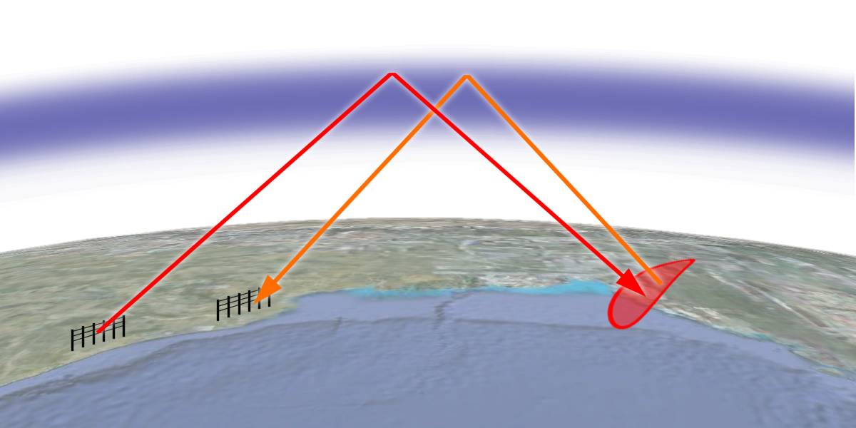
I could go into how OTHR works, but it’s been covered elsewhere in extreme detail. One of the best places for a basic overview is Wikipedia, where the image below is taken from.
How a skywave OTH radar works: A powerful shortwave signal from a large transmitting antenna (left) reaches a target beyond the horizon by reflecting off the ionosphere, and the echo signal from the target (right) returns to the receiving antenna by the same route. Image by Charly Whisky. More information on OTHRs is available on Wikipedia
Konteyner specifics
Officially designated Object 5452, construction work of the original transmitter and receiver sites commenced in 2000, taking two years to complete.
The Konteyner receiver site, with one array, was situated 6 km to the South West of Kovylkino, whilst the transmitter site – also with one array – was located 5 km north of Gorodets in Nizhny Novgorod Oblast. The system covered airspace to the west of Russia with a central bearing of 275 degrees, arcing out in a fan, with an approximate range of 3000 km (depending on radar pulse rates – covered later). Due to Ionospheric bounce a null area is created that is approximately 900 km in depth from the transmitter site. Here, nothing would be picked up by the Konteyner systems, and other OTHRs such as Resonans-N and standard Air Defence radar systems are used to fill in these gaps.
Gorodets transmitter site on 25/10/16
However, the Gorodets site is no longer in use, despite many blogs and expert publications saying otherwise – Jane’s included (until my article). Located at 56°41’34.1″N 43°29’11.3″E, this site has been dismantled since at least 6/2/18 according to Google earth imagery. All the concrete footings remain, but the antenna array is no longer there.
Gorodets transmitter site as it is now.
The receiver site at Kovylkino is still there, and from June 2016 construction had begun on two other receiver arrays, creating a triangle. Array one continued to cover a 275-degree bearing whilst the new arrays covered 155 degrees and 215 degrees.
Kovylkino receiver site with the original first array on the West.
Each receiving array contains 144 masts, all approximately 34 metres in height. They are split into three sections where the two outer ones – consisting of one group of 23 masts and the other of 24 – is between 300 and 310 metres wide. Each antenna here has 14 metres of spacing between them. The inner section contains the remaining 97 masts with 7 metres between each. The total length of the array is over 1.3 km.
Matching these receiver arrays was a new transmitter site just 15km to the South East. Imagery on Google Earth from 29/6/16 shows that there are three arrays being constructed in a Y pattern, each with the same three bearings as the receiver site. By 18/8/17 it is clear that the southern array originally thought to be covering 275 degrees instead covers 095 degrees. A second array is visible being built back to back with the 095 array to cover 275 degrees. Moreover, this meant that the original 275 degree receiver array was also being used by both transmitters.
Kovylkino transmitter site with many areas still under construction
The closeness of the transmitter site to the receiver site for long range OTHR systems is a strange one. In general they are a good 100 kilometers apart – the Australian JORN system is good example of this. Moreover, putting all the arrays so close to each other – at both sites – opens the whole system up to being destroyed, or put out of action, by just one air strike!
Each transmitter array has up to 11 generator buildings located to the rear of the antennas. Four of these buildings are also located at the original 095/275 degree receiver array. Google Earth imagery from 24/2/18 shows both sites still under construction. From 1st December 2018, combat testing of Konteyner had started and satellite imagery shows all four arrays to have generators in place by November 2018.
Generator buildings situated to the rear of the 095/275 receiver array. These appear to be the same as the 11 situated at each transmitter array.
The transmitter site consists of 44 masts in a line, 500 metres in length. The masts themselves are of differing height with the 22 tallest ones approximately 34 metres tall. The remaining 22 are approximately 25 metres in height. The masts are split up into groups of 11 of each kind.
095 bearing transmitter array at the new Kolvykino site, with the footings in place for the 275 degree array
With ranges of over 3000 km for each transmitter – effectively there are four OTHRs in use – the number of radar tracks that are captured will be in their thousands, many of which are civilian. Moreover, static features such as large buildings are also captured, showing as background noise or unknown tracks.
There are two methods used to eliminate the background noise. Firstly, during testing many of these will show through time and are deemed static and can be filtered out. Secondly, this type of OTHR – known as OTH-B or Over-the-Horizon Radar (Backscatter) – employ a Doppler effect to distinguish between static and moving targets requiring fast computers with high processing power. Doppler uses frequency shift created by moving objects to measure their velocity and so can track targets travelling at any speed, even down to 1 or 2 knots for ship traffic. Whilst older Russian OTHRs – and likely Konteyner in its early days – would have struggled in this area, modern computers can cope with the Doppler methodologies used. Anything deemed not moving by the Doppler effect can be eliminated as a potential threat or track, and are also filtered out.
To further eliminate any overloading caused by unwanted tracks, areas of interest are set up within the radar coverage which are then further split into smaller areas or “search boxes” where radar returns outside of these are ignored. These search boxes can be moved by operators as required.
The radar system is unable to determine any height parameters therefore each track is just a target at an approximate GPS position, and could be on the ground or anywhere up to 100 km in altitude! In other words, it is the equivalent to a primary track in the standard radar world. Moreover, each track could be displayed at an operators console with a radar return that depicts the target to be kilometres in size! This further complicates determining the actual location of the track.
Finally, OTHR technology does have another drawback that is much harder to filter out. Just by looking at the images below you can see that a substantial number of aircraft tracks are still captured within the search boxes, particularly in busy airspace such as around airports and heavily used civil ATC airway systems.
Here, a screengrab of a video release from 1st December 2019 when Konteyner went live shows the four areas covered by the four OTHRs, which then have search boxes at areas of interest.A close up from the video, here showing Lt. General Andrei Demin, Commanding Officer of the 1st Air Defence Division, provides a better view of the search boxes from the 215 degree array. This antenna array obviously set up to cover the Black Sea region and Mediterranean Sea. The search boxes appear to only show air traffic, though Konteyner has the potential to pick up shipping too, and it clearly shows the busy airspace around Istanbul. It is highly likely that this area was selected for the search boxes to highlight the OTHRs potential at picking up traffic, but also to NOT show what it can pick up in the Med.
One thing that OTHR doesn’t have is an Identification Friend or Foe (IFF) capability. Without IFF, this then makes it even harder to determine who is friendly, who is just an airliner or who is a potential threat.
Each of these tracks needs to individually interrogated and the routes plotted to eliminate the potential threat. For instance, all traffic into Istanbul pictured above tends to fly the same routes in and out of the airport there, so whilst the track can’t be fully removed from the display (or filtered out) it can be “ignored”. If IFF was an OTHR capability – and this is the same for other OTHR systems, not just Konteyner – then known transponder codes allocated to airports/airway systems etc. could then be filtered out. This happens in everyday ATC operations where certain transponder codes can be filtered out to remove clutter at the press of a button.
This then can make OTHR monitoring reasonably labour intensive for operators covering areas of high aviation activity despite modern computer technology being there to help.
OTHR range capabilities are controlled by the pulse rate of the signal sent by the transmitter site. In general, Konteyner operates at 50 pulses per second (pps) giving a range of approximately 3000 km. This pulse rate is also used by many other OTHRs such as the Australian JORN system (Jindalee Operational Radar Network).
Another screenshot taken from the media video at the operational handover of Konteyner showing the standard range of approximately 3000 km from Kovylkino, Mordovia.
OTHR has a potential advantage over standard radar systems in that it can track stealth aircraft such as USAF B-2s and F-35s. JORN reportedly tracked a USAF F-117 Stealth in the 1990’s that was on a round the world flight proving it couldn’t be picked up by radar! The Royal Australian Air Force (RAAF) were so confident they’d tracked it, they gave the details of positions the F-117 took to the USAF. I couldn’t find any confirmation on this from USAF documentation but it is possible.
By using the Ionospheric HF bounce, the radar is effectively looking down on top of the aircraft rather than at a very low angled Microwave radar signal head on to the target. This creates a larger return and using Doppler frequency shift is able to establish whether the track is moving, and at what speed. An early heads-up of a potential stealth bomber attack on Russia gives them the advantage of knowing where to send intercept aircraft and set up other defence methods. In the case of an ICBM strike, extra vital minutes warning can be provided. But, as previously mentioned, the position isn’t 100% accurate and can only provide an approximate location of the target – the system can not be used for any weapons fire control.
Konteyner signal received using an AirSpy HF+ Discovery SDR in high resolution with SDR# softwareClose up of same signal. Due to the high resolution, the individual pulse sweeps can not be seen and are instead show as a blurred pattern.
As previously mentioned, in general Konteyner uses a 50 pps radar signal sent as frequency modulation on pulse (FMOP) using an approximate 12 to 14 kHz of bandwidth. However, through analysis of the Konteyner signals other pps rates of 25 and 100 have been recorded giving ranges up to 6000 km and 1000 km respectively. The manufacturer of Konteyner, NPK NIIDAR (Scientific and Research Institute for Long-Distance Radio Communications), has confirmed the 3000 km range, along with an altitude coverage of 100 km.
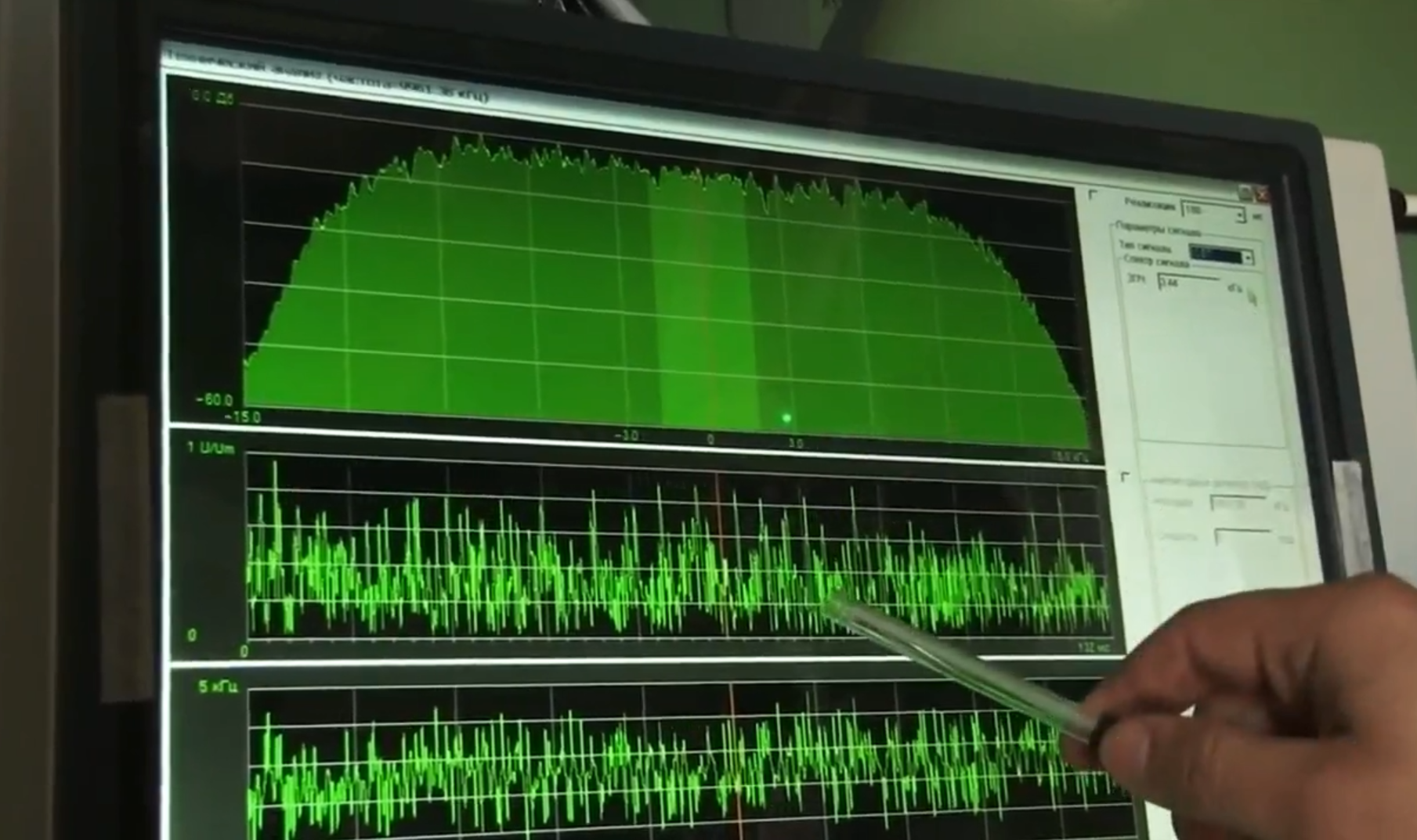
When analysing the signal in Procitec’s go2MONITOR software, the pulse sweeps can be seen much clearer, though still at this resolution there is a blurring to the sweeps. The software has automatically ascertained the sweep rate of 40 Hz – or 40 pps – at a bandwidth of around 12 kHz. A 40 pps sweep for Konteyner provides a radar coverage range exceeding the stated 3000 km – up to approximately 4000 km.
One find in my analysis of Konteyner signals was quite interesting.
Quite often when analysing OTHR signals closely, you can see weak Back-scatter return signals between the main pulses. These weak signals travel in the same radar sweep direction as the transmitted ones in either a down-sweep mode from a high frequency to a low one, or in an up-sweep mode from to low to high.
In the image below though you can see another, weaker, radar pulse emanating from the point the first down-sweep pulse ends, travelling up in frequency range and creating a V. If you look closely you can also see a very weak back-scatter signal from both.
My conclusion from this is that the up-sweep pulse is from the 095 degree Konteyner transmitter array, whilst the stronger down-sweep one is from the 275 degree array – the stronger signal is in theory pointing at my antenna in the UK and hence would be emanating from the 275 degree array.
The fact that this signal comes from the 095/275 arrays is a guess of course but I think I’m right. I am also going to guess that the complete radar pulse for the 095/275 transmitters starts at one end of one array, travelling along the 44 masts. When this pulse ends the other array starts in the opposite direction. Moreover, with this method there should be zero interference between the two arrays as they wont be transmitting at the same time.
In the image above, taken from from a screen grab of Procitec’s go2DECODE, you can see that each pulse is every 25 ms, therefore confirming a rate of 40 pps – the software also determines this automatically as shown in the table to the right. Also of note is the analysed signal in the frequency window (Hz) at the bottom. Here you can clearly see the V created by the two pulses.
When we look at the Time display window in go2DECODE (shown below) we can see that I’ve measured the total length of both pulses to be around 6.5 ms. But on closer inspection I think I’ve cut that short a little and it should be 8 ms. This would mean each pulse lasts 4 ms and ties in nicely with the 25 ms per pulse gap as there’s a 21 ms spacing between the end and start of each individual pulse.
I also wonder, that with a gap of 17 ms between the end of the second pulse and the beginning of the first one again, in theory there’s enough of a gap to fit two more 4 ms pulses between these from the the two remaining Konteyner arrays transmitting at 40 pps. Even at a higher 50 pps rate, the 12 ms gap is enough to allow the two remaining pulses to take place with a 4 ms buffer.
This then means that all four Konteyner transmitter arrays can be operational at the same time without causing any potential interference to each other, whether they use the same frequency or different ones. In this case, I’ve been lucky to capture two of the arrays using the same frequency – well, I think I have 🙂
Nevertheless, monitoring the Konteyner signals should bring some further interesting finds, especially if they are using the same frequency occasionally for different surveillance areas. Moreover, it would also be interesting to find all the various pps rates so that system ranges can be established.
Whilst for many, OTHR signals are a pain, wiping out other signals, they still have a lot to give when it comes to SIGINT gathering.
And it may not end at just the one Konteyner system. On the 1st December 2019 it was also announced that a further system would be activated to cover the Arctic region. At the moment, any potential sites have not been mentioned or found, but a likely site would be near Severodvinsk in the Arkhangelsk Oblast, or near Severomorsk in the Murmansk Oblast. Both of these are close to the 1st Air Defence Division headquarters located in Murmansk. My only negative thoughts on this would be that these sites are too close to areas of interest because of the ionosphere skip created, and also probably too far north – ionospheric bounce is not so good towards the poles.
As the original Konteyner transmitter site seems to be being maintained still, be it without any antennas, it also has the interesting aspect of being around 900 km south of the White Sea and areas of coverage needed – perfect for the ionospheric skip. Could this site be changed in aspect so that a transmitter array points to the north to cover the White Sea, Barents Sea and the northern Island? There’s certainly enough room to do this at the Gorodets site.
There has also been mention of another Konteyner site already in construction in the far east. At this time nothing has been found of any construction site that looks to be a Konteyner OTHR and I have my doubts about this. It was first muted in 2010, then again in 2018, and I would have expected something to be there by now.
I highly suspect that this plan has been abandoned, and the 095 degree OTHR of the Kovylkino Konteyner site has taken over the far east coverage.
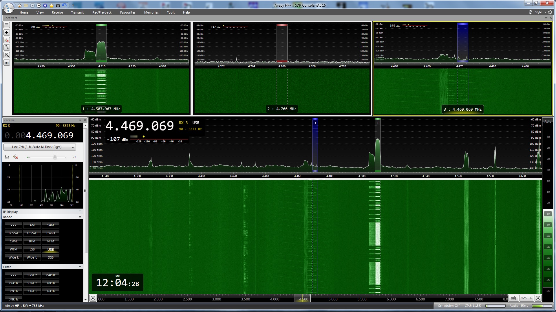
In early November, whilst working on an article for Janes, I noticed a Link-11 SLEW signal on 4510 kHz (CF) that was slowly growing in reception strength. I’d been monitoring frequencies used by the Northern Fleet of the Russian navy around this one and had already spotted that Link-11 CLEW was being used on a nearby frequency, though this remained at a constant signal strength at my location. The fact that the Link-11 SLEW was getting stronger made me stop what I was doing and start concentrating on this instead.
AirSpy HF+ Discovery SDR with SDRConsole operating software. Link-11 SLEW signal in Receiver 1, and the weaker Link-11 CLEW signal in Receiver 3. Whilst there a two SLEW signals showing, there is just one, with the left hand one being produced by the strong signal. You can see the weaker transmissions from a receiving station between the stronger ones on the correct frequency, but not on the “reflection”.
Link-11 SLEW (Single-Tone Link-11 waveform) ,or STANAG 5511, is a NATO Standard for tactical data exchange used between multiple platforms, be it on Land, Sea or Air. Its main function is the exchange of radar information, and in HF this is particularly useful for platforms that are beyond line of sight of each other and therefore cannot use the UHF version of Link-11.
With propagation being the way it is, in theory radar data could be exchanged between platforms that are hundreds to thousands of miles apart, therefore providing a wider picture of operations to other mobile platforms and fixed land bases. This data can also be forwarded on using ground stations that receive the data and then re-transmit on another frequency and/or frequency band. However, the approximate range of an individual broadcast on HF is reported to be 300nm.
As well as radar information, electronic warfare (EW) and command data can also be transmitted, but despite the capability to transmit radar data, it is not used for ATC purposes. In the UK, Link-11 is used by both the RAF (in E-3 AWAC’s and Tactical Air Control Centres) and the Royal Navy. Primarily it is used for sharing of Maritime data. Maritime Patrol Aircraft (MPA’s) such as USN P-8’s and Canadian CP-140’s use Link-11 both as receivers and transmitters of data, so when the RAF start using their P-8’s operationally in 2020 expect this to be added to the UK list. Whilst it is a secure data system, certain parameters can be extracted for network analysis and it can be subjected to Electronic Countermeasures (ECM).
Link-11 data is correlated against any tracks already present on a receivers radar picture. If a track is there it is ignored, whilst any that are missing are added but with a different symbol to show it is not being tracked by their own equipment. As this shared data is normally beyond the range of a ships own radar systems, this can provide an early warning of possible offensive aircraft, missiles or ships that would not normally be available.
I started up go2MONITOR and linked it to my WinRadio G31 Excalibur. Using a centre frequency of 4510 kHz I ran an emission search and selected the Link-11 SLEW modulation that it found at this frequency.
It immediately started decoding as much as it could, and I noticed that three Address ID’s were in the network.
go2MONITOR in action just after starting it up. Note, three ID’s in the network – 2_o, 30_o and 71_o
As the signal was strong, and it is normally maritime radar data that is being transmitted, I decided to have a quick look on AIS to see if there was anything showing nearby. Using AISLive I spotted that Norwegian navy Fridtjof Nansen class FFGHM Thor Heyerdahl was 18.5 nm SW of my location, just to the west of the island Ailsa Craig. Whilst it was using an incorrect name for AIS identification, its ITU callsign of LABH gave me the correct ID. This appeared to be the likely candidate for the strong Link-11 signal.
Position of Thor Heyerdahl from my AIS receiver using AISLive software
It wasn’t the best day and it was pretty murky out to sea with visibility being around 5nm – I certainly couldn’t see the Isle of Arran 11.5 nm away. I kept an eye on the AIS track for Thor Heyerdahl but it didn’t appear to be moving.
Whilst my own gear doesn’t allow me to carry out any Direction Finding (DF) I elected to utilise SDR.hu and KiwiSDR’s to see if I could get a good TDoA fix on a potential transmitter site – TDoA = Time Difference Of Arrival, also known as multilateration or MLAT. Whilst not 100% accurate, TDoA is surprisingly good and will sometimes get you to within a few kilometres of a transmission site with a strong signal.
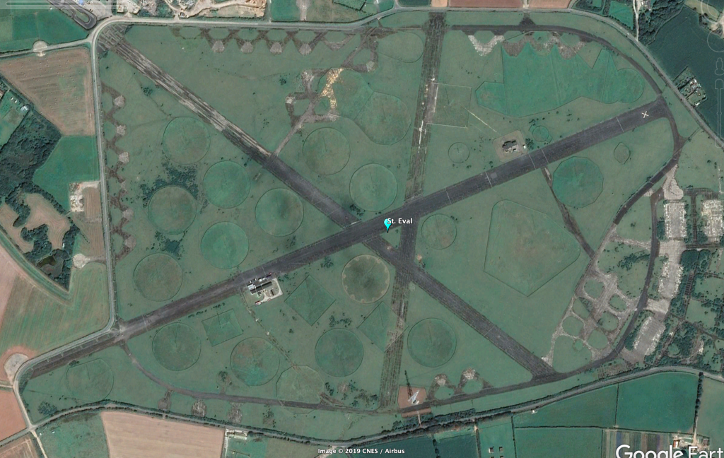
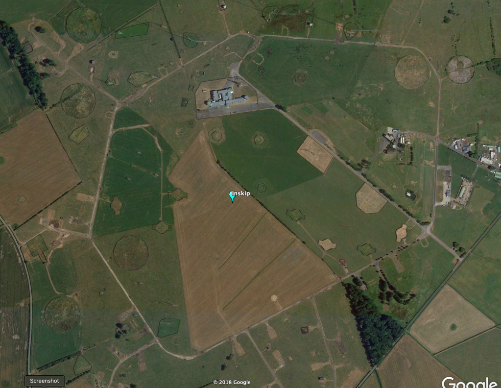
One of my thoughts was that the signal was emanating from the UK Defence High Frequency Communications Service (DHFCS) site at either St. Eval in Cornwall or Inskip in Lancashire. With this in mind I picked relevant KiwiSDR’s that surrounded these two sites and my area and ran a TDoA.
As expected, the result showed the probable transmitter site as just over 58 kilometres from St. Eval, though the overall shape and “hot area” of the TDoA map also covered Inskip, running along the West coast of England, Wales and Scotland. It peaked exactly in line to where the Norwegian navy ship and I were located! With the fact that there were signals being received from three different sources it is highly likely this has averaged out to this plot.
TDoA result showing the likely transmitter site at 50.60N 4.20W. Note the elongated “hot spot” which denotes the area that the transmitter site is likely to be situated.
Just after 10am the weather cleared allowing me to see a US Navy Arleigh Burke class DDGHM between myself and Arran. This added an extra ship to the equation, and also tied in with the TDoA hot spot. Things were getting even more interesting!
Link-11 SLEW at its strongest which also coincided with USS Gridley being its closest to my location.
Thor Heyerdahl still hadn’t moved according to AISLive but the Arleigh Burke was clearly heading in to the Royal Navy base at Faslane. With my Bearcat UBC-800T scanning the maritime frequencies it wasn’t long before “Warship 101” called up for Clyde pilot information along with an estimate for Ashton Buoy of 1300z. Warship 101 tied up with Arleigh Burke USS Gridley.
The Link-11 SLEW signal was considerably weaker at the time USS Gridley was at Ashton Buoy.
As USS Gridley progressed towards Faslane, the signal started to get weaker. Ashton Buoy is where most ships inbound for Faslane meet the pilot and tugs, taking up to another 30 minutes to get from there to alongside at the base – a journey of about 8.5nm.
At 1328z the Link-11 SLEW signal ended which coincided with the time that USS Gridley approached alongside at Faslane. It would be at about this time that most of the radar systems used on the ship would have been powered down so data was no longer available for transmission, therefore the Link-11 network was not required any further and it was disconnected.
Some images of USS Gridley arriving into Faslane taken by good friend Dougie Coull
So, was this Link-11 SLEW connected to USS Gridley? And was the ship also the NCS of the network? I think the answer is yes to both, and I’ll explain a couple of things that leads me to this conclusion. But first…………….
Link-11 SLEW Technical details
Using Upper Side Band (USB) in HF, a single waveform is generated in a PSK-8 modulated, 1800 Hz tone. The symbol rate is 2400 Bd and the user data rate is 1800 bps. Link-11 SLEW is an improved version of the older Link-11 CLEW modulation and due to enhanced error detection and correction is a more robust method of sending data. This makes it more likely that transmissions are received correctly the first time. Moreover, an adaptive system is used to counter any multipath signals the receiving unit may experience due to HF propagation.
The waveform transmission consists of an acquisition preamble followed by two or more fields, each of which is followed by a reinsertion probe. The field after the preamble is a header field containing information that is used by the CDS (Combat Data System) and an encryptor. If a network Participating Unit (PU) has any data, for instance track data, this follows the reinsertion probe. Finally, an end-of-message (EOM) is sent followed by a reinsertion probe.
The header is made up of 33 data bits and 12 error detection bits (CRC – Cyclic Redundancy Check). The 45 bit sequence is encoded with a 1/2 rate error correction code therefore giving a 90 bit field. The header contains information on the transmission type used, Picket/Participating Unit (PU) address, KG-40 Message Indicator, the NCS/Picket designation and a spare field.
Broken down, each piece of information is made up as follows:
The transmission type indicates the format of the transmission – 0 for a NCS (Network Control) Interrogation Message (NCS IM); 1 for a NCS Interrogation with Message (NCS IWM) or a Picket reply.
The address contains either the address of the next Picket or that of the Picket that initiated the call.
The KG-40 Message Indicator (MI) contains a number sequence generated by a KG-40AR cryptographic device. Synchronization is achieved when the receiver acquires the correct MI. For a NCS IM this will be made up of zeros as no message or data is actually sent.
The NCS/Picketdesignation identifies whether the current transmission originates from the NCS or PU: 0 = NCS; 1 = PU
Following on from the header, the SLEW data field consists of 48 information data bits along with 12 error detection and correction bits, themselves encoded with 2/3 rate error correction. This creates a 90 bit data field.
The EOM indicates the end of the transmission and is also a 90 bit field. There are no error detection or correction bits. Depending on the unit that is transmitting, a different sequence is sent – NCS = 0’s; PU = 1’s
Analysis
There is a specific order of transmissions which takes place for data to be exchanged.
Ordinarily the NCS sends data that creates the network, synchronizing things such as platform clocks etc. Each PU is called by the NCS and any data that a PU has is then sent, or the NCS sends data, or both. This is a very simple explanation of how data is exchanged but if you monitor a SLEW network you’ll see the exchanges take place rapidly. Except for the message itself which is encrypted, go2MONITOR will decode all the relevant information for you for analysis. This means that you don’t need to look at each raw data burst as sent to calculate whether it was a PU reply or NCS IWM, the decoder will do this for you.
At this point I need to say that Link-11 decoding is only available in the Mil version of go2MONITOR so doesn’t come as standard. Should you be interested in Link-11 decoding yourself then you would need to go for the full go2MONITOR package to enable this.
As previously mentioned, the data itself is encrypted but it is possible to try to calculate who is who within the network, and the analysis of the header information in particular will give you a good clue if you already know of potential PU’s that could be on the frequency.
In this case we already have four possible PU’s:
USS Gridley
Thor Heyerdahl
St. Eval transmitter site
Inskip transmitter site
It later transpired that Thor Heyerdahl had gone into Belfast Harbour for repairs so this practically cancelled out this ship as the NCS though it could still be a PU. Moreover, Thor Heyerdahl and USS Gridley were part of the same NATO squadron at that time which meant it was highly likely they were on the same network. This left us with three choices for the NCS, but still four for the network.
Here, I’d cancel out Inskip completely as both the NCS and a PU as the TDoA appeared to give a stronger indication to St. Eval – that left us with three in the network.
The pure fact that the strength of the major signal increased as USS Gridley got closer to my location, then slowly faded as she went further away added to my theory of her being the NCS. This was practically confirmed when the signal stopped on arrival to Faslane. Throughout the monitoring period he other signals on the frequency remained at the same strength.
Based on this, this meant that the strong signal was USS Gridley using ID Address 2_o.
Let’s take a look at one the previous screenshots, but this time with annotations explaining a number of points.
Firstly, we need to look for the NCS. The easiest way to do this is to look at the NCS/Picket Designation and find transmissions that are a zero, combined with a Message Type that indicates it is a NCS IWM. Here, there is just one transmission and that emanates from Address ID 2_o – the long one that includes a data message.
We next need to find NCS/Picket Designation transmissions that still have a zero – therefore coming from the NCS – but that have a Message Type that show it to be a NCS IM. These are calls from the NCS to any PU’s that are on the network looking to see if they have any “traffic” or messages.
Because of this there should be numerous messages of this type, and if you notice none have an ID address of 2_o. However, all of these messages are actually coming from 2_o as the ID address shown in a NCS IM is that of the PU being called rather than who it is from.
Any reply messages from PU’s will show as a NCS IWM/PU Reply transmission, but importantly the NCS/PU designation will be a one – showing it isn’t the NCS. Here there is one data reply from 71_o. You’ll notice that in the “reflection” there isn’t any transmission, unlike the ones from 2_o.
Moreover, though not shown here as the messages were off screen and not captured in the screen grab, you can see that one of the PU’s sent another reply message. As I was able to look at the complete message history I was able to see that this was also from 71_o – and 2_o either replied to this or sent further data.
There are two fainter transmissions which were not captured by go2MONITOR. These were from a PU, and must have been 30_o as there are no transmissions at all in the sequence that are from this ID address.
We now have a quandry. Who was 30_o and who was 71_o?
Data is definitely being sent by 71_o so to me this is more likely to be a ship rather than a transmitter site – but – a strong TDoA signal pointing at St. Eval makes it look like 71_o is this location instead.
Now though, we need to think outside the box a bit and realise that I’m looking at two different sources of radio reception. The TDoA receivers I selected were nowhere near my location as I’d selected KiwiSDR’s that surrounded St. Eval. This meant the signal that was weak with me could have been strong with these, therefore giving the result above.
If I base the fact that I think USS Gridley is 2_o due to strength, then I must presume the same with 71_o and call this as Thor Heyerdahl as this is the second strongest signal. I can also say that having gone through the four and a half hours of Link-11 SLEW transmissions available that 30_o never sent a single data transmission – or rather, not one that was received by me.
Full four and a half hours of Link-11 SLEW as shown in the go2MONITOR results page. You can see other areas (in red) that I was decoding at the same same. By selecting an area in the results page you can access the data as decoded, saved into files. I could have further enhanced this and carried out a full audio recording for further analysis, but I didn’t on this occasion.
Here then is my conclusion:
USS Gridley = 2_o and the NCS
Thor Heyerdahl = 71_o
St. Eval transmitter site = 30_o
Of course, we’ll never really know, but I hope this shows some of the extra things you can do with go2MONITOR and that it isn’t just a decoder. It really can add further interest to your radio monitoring if you’re an amateur; and if you’re a professional with a full plethora of gear, direction finders, receiver networks etc. then you really can start getting some interesting results in SIGINT gathering with this software – and highly likely be able to pinpoint exactly who was who in this scenario.
Now, how do I get some Direction Finders set up near me….Hmmmmmm??
If you follow me on Twitter you’ll see that in the last month or so I’ve been sending out images of classification and decoder software go2MONITOR working with a number of my SDR’s.
go2MONITOR is part of the go2SIGNALS range of software solutions created by PROCITEC GmbH operating from Pforzheim in Germany, themselves part of the PLATH group. PLATH Group is the leading European-based solution provider for communication intelligence and electronic warfare (EW) with worldwide government customers. The group covers all aspects of signal interception and analysis split between a number of companies such as PROCITEC. EW, COMINT/SIGINT, Jamming and Decoding are just a small part of what the group specialises in.
go2MONITOR is advanced high-performance, automatic HF, VHF and UHF monitoring software capable of recording, SDR control, wideband and narrowband classification and multichannel signal decoding.
It isn’t for the faint hearted, but once you get used to using it, it really does make gathering information on networks extremely easy. And it decodes many modes other software can’t.
In a series of blogs I’m going to show you the capabilities of this amazing software, though I must stress now, it is aimed at Professional SIGINT gathering and it comes with a Professional price tag.
Saying that, it doesn’t mean it isn’t available to the non-professional. It is open to all and to cover this it comes in various versions starting with the Standard package progressing to a full Military package – which gives you the full range of HF, VHF and UHF classification and modem recognition decoders available, including PMR and SAT (Inmarsat AERO). The Standard version isn’t to be sniffed at, it still gives you an amazing range of decoders, though you could easily argue that many of these are available in other free – or near to free – decoding software like MultiPSK or Sorcerer. A full list of decoders available can be found here. Note, this list is broken down into the various packages and not all are available with the Standard option. Confirm what belongs to what if you’re thinking of purchasing.
Various signals within the Satellite L-band using an AirSpy R2 and SDR#
So what’s the difference in what go2MONITOR can do with other software available? That’s the idea of these blogs, to answer just that question. It will take quite a few blogs – mainly because there isn’t just one answer.
Here then, is a brief overview of what can be done, what SDR’s it works with – in fact, not just SDR’s but all receivers that can produce a recording – and any other things I can think of.
As, I’ve said then, it can decode pretty much any data signal out there. Obviously, some signals are encrypted so it wouldn’t fully decode unless you had the key, but you can get the encrypted messages. It can also classify voice signals, not just data. So, if you wanted to hunt out various voice networks, go2MONITOR can assist you in doing this.
Here is where it excels. Classification – and doing it very quickly.
Imagine being on your SDR (SDR1) and you can see a whole load of data signals on the waterfall/spectrum and you quickly want to know what they all are. With go2MONITOR operating another SDR (SDR2) you can dial in the centre frequency of the bandwidth shown on SDR1 into the go2MONITOR/SDR2 combo, click one button – Find Emissions – and within seconds the whole bandwidth has been analysed and every signal classified.
I’ll go back a step though here. You don’t need two SDR’s. One will do. SDR1 – as long as it is a compatible SDR – can be controlled through a GUI by go2MONITOR. The software includes a waterfall/spectrum display. Like all SDR software, these displays are fully adaptable to how you like to see the signals.
The previous L-band bandwidth but his time using go2MONITOR and the AirSpy R2 GUI, decoding INMARSAT 3-F2
Either way, you now have a list of every emission that go2MONITOR has received within that bandwidth. This list includes Modulation type, Frequency, Bandwidth, Symbol (Baud) rate and SNR. It also shows which SDR you have used for interception (useful if you’re using go2MONITOR with more than SDR at the same time, but also with other advanced features such as network control), and it also shows if the frequency is already stored within the frequency database – yes, you can create this too; or import ready made databases in a CSV format.
All the emissions within the bandwidth have been analysed and types ascertained.
Already then, you have built up a picture of what these signals are. One thing to note. If the signal type is not one of those included within the package you have, it will be classed as unknown. Example – a STANAG 4285 will show as unknown in the Standard and PMR/SAT package, but will be classified correctly in the MIL package.
OK, those of us that are looking at SDR’s all the time can pretty much tell what the signals are just by looking at them, so there’s no great advantage here is there? Except, now go2MONITOR has logged these in its database which can be searched through at a later date – handy if you’re looking for potential schedules for example.
However, the next step is where things get interesting. By putting one of these emissions into a “Channel” you can carry out an advanced classification, recognition and decode. You have multiple choices here, but I generally start off with a Classification. Whilst the software has already decided what the emission type is, by doing this it double checks just this one channel and produces a choice of decoders that it is likely to be.
go2MONITOR in Classification mode. Here it has calculated that the FSK emission received has a 50 Bd symbol rate with two tones with 859 Hz spacing. From this it has deduced it is likely to be one of four modems – one of which is ALE-400.
By using STANAG 4285 as an example, it will put this into the list of choices, but it may put other PSK signals there too. By clicking on another button, this puts the channel into Recognition mode and it reduces the hundreds of decoders down to just those in the classification list produced. The software then calculates which is the best decoder and starts to decode the signal.
If you think about STANAG 4285 in other software, you generally have to try all the various potential Baud rates – is it Long Interleaving? is it Short? etc etc. Well go2MONITOR does this automatically. It checks the alphabet and protocol and will decode it if known. More often than not it can’t calculate the alphabet, but every now and again it does and it will produce encrypted data – don’t forget, if it’s encrypted it won’t decrypt it without the correct key.
By continuing on the process from the Classification mode into the Recognition & Decode mode, here from another emission go2MONITOR has selected the CIS-50-50 modem and started to decode the message.
This further Recognition and Decoding is also stored in the database for later analysis, along with a recorded wav file for playback and deeper signal analysis.
Seriously, it is harder describing it in text than it is doing it so I’ve created a video that’s at the end of this blog.
I mentioned previously that the software works with receivers that aren’t SDR’s. That’s because, as long as you can create a wav file recording – Narrowband as it’s known in go2MONITOR – it can be analysed. There are things missing, the actual frequency for instance (though this can be typed into a text box so that you can then have the right information – this i’ll show in a later blog). Time stamps aren’t naturally there but again you can add these by telling the software to use the time the recording was started.
I’ve used recordings made on my Icom IC-R8500 as an example of this but it is literally the bandwidth of the mode used by the receiver that is shown on the go2MONITOR spectrogram.
You don’t actually need to own a receiver of your own. Use an online SDR such as a KiwiSDR, record the IQ as a wav file and play it back through go2MONITOR for analysis. I’m doing just that for a Jane’s Intelligence Review magazine article.
If you use SDRConsole, then you may have also tried the File Analyser function that I blogged about in August last year. The File Analyser in SDRC is excellent, there’s no doubt about it, but it has one drawback. Once you’ve carried out your recording you have to create a run through of the recording, making an XML file that effectively joins all the wav files up. If you’ve made a wide and long IQ recording this can take quite some time. With most of my overnight recordings – normally 7 hours long, with a 768 kHz bandwidth – this takes around 45 minutes to complete.
With go2MONITOR you can also record the bandwidth IQ data. With this you can do two things. Firstly you can run it through as a normal playback, classifying and decoding as you go. Secondly though, you can open the Results window which gives you a time based view of the whole recording allowing you to immediately see any transmissions. Unlike SDRC Analyser, the signals have already been classified, and more importantly, this is done straight away without any need to create an XML file first. The Results window will be covered in greater detail in a blog of its own.
Analysing a Wav file made using the IQ recording capabilities with go2MONITORFurther analysis of a STANAG 4285 emission within the recording.
However, there are no decodings here. With just an IQ recording you need to play it back and run an emission search etc. There are some basic automation tasks available, such as setting up an emissions search every 10 seconds.
But, if you have the Automated Monitoring and Tasking package, you can also have the software automatically record, recognise and decode a single emission type – or all emissions types within the bandwidth, a set frequency, between two frequencies or any other parameters you may wish to set up.
The go2MONITOR results window of a IQ recording that has been set up to automatically run an emissions search every 10 seconds. The blue rectangles are every emission found. By running the mouse of them you can get basic information on each emission. Clicking on them brings further details that can be viewed in the tabbed area to the right.The red rectangles are emissions that have also been Recognised and Decoded. By clicking on them the decoded data is shown in the tabbed area.
The list of SDR’s that can be used with go2MONITOR is pretty good, though due to the target audience, many of them are high end, “government/military” receivers. But, it does work with Perseus, SDRplay RSP1 & RSP2, RFSpace NetSDR and SDR-14, and of course AirSpy R2 – and now the AirSpy HF+ and AirSpy HF+ Discovery.
Supported receiver list:
Receiver
Max. Rx bandwidth
Spectrum overview
Scan
Remark
AirSpy
2 MHz
Experimental support
CommsAudit CA7851
5 MHz
VITA 49
Grintek GRX Lan
1 MHz
IZT R3xxx series
20 MHz
X
X
Up to 3 channels spectrum
IZT R4000 (SignalSuite)
1 MHz
1 channel only
Microtelecom PERSEUS
800 kHz
Limited USB 3.0 compatibility
narda® NRA-3000 RX
320 kHz
narda® NRA-6000 RX
320 kHz
narda® IDA 2
320 kHz
narda® SignalShark®3310
20 MHz
VITA 49 support. Only 1 MHz and no receiver control at LINUX
PLATH SIR 2110
20 MHz
LINUX recommended. External receiver control only
PLATH SIR 2115
4×20 MHz
External receiver control only
PLATH SIR 5110
12 MHz
16×768 kHz subbands External receiver control only
PLATH SIR 5115
Full HF
40×768 kHz subbands External receiver control only
R&S EB500
5 MHz
X
No gain control available
R&S EM100 / PR100
500 kHz
X
X
R&S ESMD
15 MHz
External receiver control only
RFSPACE NetSDR
2 MHz
RFSPACE SDR-14
190 kHz
RTLSDR/Noxon USB-sticks
3.2 MHz
Experimental support. Continuous signal up to 2.4 MHz
SDRplay RSP1 & RSP2
6 MHz
Experimental support
ThinkRF R5500-408
6.25 MHz
VITA 49
ThinkRF R5500-427
6.25 MHz
VITA 49
ThinkRF WSA5000-408
780 kHz
VITA 49
ThinkRF WSA5000-427
780 kHz
VITA 49
WiNRADiO G31DDC
800 kHz
WiNRADiO G33DDC
4 MHz
X
WiNRADiO G35DDC
4 MHz
X
WiNRADiO G39DDC
4 MHz
X
Up to 2 channels + spectrum
Generic VITA 49 receiver support
Max. receiver bandwidth
Can be configured in a wide range for different receiver types
Other generic “Winrad ExtIO” supported receivers
Max. receiver bandwidth
Experimental support
As you can see, there is a huge difference in bandwidth capabilities for each receiver. I use my WinRadio G31DDC quite often with go2MONITOR, but the AirSpy HF+ Discovery (not listed as i’ve only just got it working) isn’t much worse with it’s full 610 kHz bandwidth.
When you think that the G31 has a much better operational bandwidth than 800 kHz when you use it on its own, it’s obvious which is better value if you were buying an SDR solely for using it with go2MONITOR. It is this kind of thing that many Government agencies are looking at when it comes to funding operations aimed at large scale monitoring.
That then is a very basic overview of go2MONITOR. The quick video and images have hopefully shown you a little of what is possible.
Outside of a Professional SIGINT operation, why would an amateur radio monitor need something like go2MONITOR? And would they pay the price?
I think they would. After all, most of us have spent a fair amount on radio monitoring over the years, so why not on software that would make their monitoring not only quicker and easier, but potentially open up new areas of monitoring.
Many of us specialise in certain monitoring areas – Russian military, particular the Navy and Strategic aviation for me for example. With go2MONITOR I have already used it to hunt out potential Russian Northern Fleet frequencies by running an automated 10 second CW emission scan overnight within a bandwidth block. By doing this, and then analysing data found in the results window, I was able to target certain frequencies to see what activity there was on subsequent nights.
Whilst there are other decoders available – some of which are plugins in software such as SDR#; some of which are free – it is the quickness and ease with which it can be done that makes go2MONITOR attractive. The big question is, would you pay for this?
Nearly two weeks ago I attended the Defence & Security Equipment International 2019 (DSEI19) at the Excel exhibition centre, London.
The intention of this blog is to provide a brief look at what I saw on the day I attended.
Generally, I was more impressed with the smaller companies that I met rather than the larger ones. The larger ones, once they’d read my name badge and saw that I was “Media”, gave me the feeling that they couldn’t wait to get rid of me as I wasn’t there to make a multi-million pound purchase from them. The smaller, or less well known, were far more attentive and provided me with a good amount of information on their products, target audience and hopes for the future.
Whilst this may turn you off from reading the remainder of the blog, I think I’ll start with the things I was a little disappointed with.
One of the companies I was extremely interested in visiting was Barrett Communications. As I’m currently writing an article for Janes on a system very much like one of their products I emailed the UK office in advance to tell them that I was coming and what I was interested in. They did reply and were keen to see I was attending, even sending me a heads up on one their new products that was yet to be revealed. I was, then, very quick to go and see them once the show started.
Barrett PRC-4090 HF Tactical Manpack. 250 kHz to 30 MHz Rx/Tx (from 1.6 MHz for Tx) – CW, USB/LSB/ISB modes – 2G/3G ALE – 10W/30W or 150W PEP depending on 12v/24v power – 5 0r 25 freq hops per second – max weight 5kg
However, once on the stand, things were very different. As I said above, the media name badge meant I wasn’t a buyer. And despite trying to show keenness on their equipment, which I’d swatted up on before attending, I got the feeling the sales chap just wanted me to leave. On a couple of occasions I was brushed aside so that he could chat or shake hands with a mate rather than carry on showing me some of their products – which are actually very good. Nice gear, not always so good at media relations.
Barrett 4050 HF SDR’s in various guises, with the capability to control via tablets such as iPads.
Unfortunately, the same can almost be said with rugged case manufacturer, Peli Products UK. This time I hadn’t emailed in advance, but I sought them out as I am actually in the market for a number of new rugged cases – a new camera case, a 13″ laptop case and a GoPro case.
Whilst this time the guy I spoke to was nice and briefly showed me their new TrekPak dividers – which are pretty cool – I got the impression he didn’t really want to be at the show and he kind of fobbed me off with a brochure rather than trying to sell me the products that I had told him I was interesting in buying. The irony here being that when you go to the TrekPak part of their website, the opening image is that of a rugged case full of camera equipment with “Press” stickers all over them.
In all honesty I could go on about quite a few other companies much like these but I don’t want to have too much of a whinge about the show, so let’s move on to the good stuff.
I obviously paid a visit to the Janes stand first, had a quick coffee and chat – and it was nice to know that they’d heard of me 🙂
Next to the Janes stand was Keysight Technologies, well known manufacturers of Signal Generators, Oscilloscopes and Spectrum Analysers – and many, many other outstanding workbench solutions. I spoke to Radar, EW and Satellite solutions manager Erik Diez, who showed me one of their solutions used to analyse an unknown radar signal with the idea of creating a potential jammer, countermeasure or signal designation. It truly was an interesting chat and the demo of the equipment was very interesting – if only any of it was within my price range 🙂 Saying that, their entry stage Spectrum Analysers etc are comparable in price to the Rigol equipment I have at home.
Keysight’s UXR0134A Infiniium UXR-Series Oscilloscope (left and on monitor) linked into other components for signals analysis. 13 GHz bandwidth and four full bandwidth channels is just part of the specifications available.
I enjoyed my time with Erik, with both of us agreeing that when I retire I may be able to buy something from him 🙂
Wondering around, there were plenty of vehicles, weapons systems, EW systems, ELINT/COMINT/SIGINT companies to take a look at. There was a huge Turkish contingent who took over a large area of the north side of the Excel with pretty much all of the above on view.
I had a chuckle to myself as I walked through an area of companies selling UAV’s, straight into another area selling various weapons and systems designed to take drones out.
As well as technical solutions there were clothing/footwear companies – I had a good chat at footwear company Rocky Boots who have some nice military boots.
BAe were there in force with various future ship models, simulators and other technologies. I even bumped into old friend Jamie Hunter on their stand – we calculated that it was over 20 years since we last bumped into each other and travelled to various bases on photo trips.
Type 26 and Hunter class models on the BAe Systems stand
I would have taken more photos of the vehicles but the stands were generally pretty close and so it made it difficult for photos. Some though I did manage:
Oshkosh Defense Joint Light Tactical Vehicle (JLTV). This vehicle will replace Humvee’s in the US forces and is already in service with the Marine Corps. The British Army also announced at DSEI that the JLTV is taking part in a two year contract to demonstrate its potential as a Multi Role Vehicle-Protected (MRV-P).The 800 Titan is on offer by Polaris Government and Defense as a militarised version of their commercial skidoos.
Polaris also had a DAGOR A1 Ultra-Light Tactical Vehicle (ULTV) on show with additional pieces of equipment added on by the likes of FN Herstal’s medium pintle mount .50 cal FN M3M
I got to play with plenty of weapons. I was very happy on the Sig Sauer stand and spent some time in the pistol area. In comparison to some of the other companies, their handguns felt good and seemed to have a smoother slide – obvs no ammo was available. I was particularly happy with the SP2022 and if given the chance to try it out properly, I’d jump at it.
A plethora of SIG Sauer hand guns, with the SP2022 nearestThere were also plenty of assault rifles and machine pistols on display, along with various sights and suppressors
On a non-live ammo front, an interesting company here in the UK is Ultimate Training Munitions – UTM. They did have a “live firing” area at the show. Instead of being live ammunition however, UTM have created training ammunition that provides a realistic environment without the potential of death. With modifications to real weapons, this ammunition can be used in exercises giving troops/law enforcement agencies the chance to fire near real ammunition at one another and know when they’ve been hit by a projectile that has a plastic cover and a coloured marker.
I’ve got to say it was very good in the small range. I feel like the next time I’m down at Mildenhall I may request a visit.
My final port of call at DSEI was the Rohde & Schwarz stand. This was for two reasons. Firstly, I wanted to spend a bit of time there as I knew their products would be very interesting and secondly – they had a bar with free Augustiner-Bräu Helles beer 🙂
The beer was great, one of my favourites on my regular visits to Bavaria. And I had a great chat with Jo who hosted me in the bar and out at the equipment on display.
R&S really do have an amazing input into many of the worlds military radio requirements. For instance, they recently provided the Royal Navy with the first land-based NAVICS radio system for the Type 26 City class FFGHM – with all ships of the class being fitted out with the integrated comms system. This will provide internal and external comms (both voice and data) via an IP network, all of which will be secure. The External VHF/UHF and HF comms will use M3SR Series 4400 and M3SR Series 4100 radios.
As well as VHF/UHF and HF comms, they will also be providing SATCOM and GMDSS systems, along with a joint venture with STS Defence for the Communication masts.
In total, the NAVICS system has been provided to over 40 navies. For the RN this includes the Queen Elizabeth class Aircraft carriers, the River class batch II patrol ships and the above mentioned Type 26’s.
Also of interest was the WPU2000 ELINT Processor, launched at the show.
The WPU2000 is a wideband processing unit – hence WPU – and has a 2 GHz instantaneous real time bandwidth. It is set out to replace the WPU500 which operates with a 500 MHz bandwidth. It collects, then processes and analyses radar signals such as those produced by low probability of intercept (LPI) radars and emissions from Active Electronically Scanned Array (AESA) radars. I was told that due to its sensitivity it can detect emmissions that may be invisible to ELINT and EW systems currently in use.
As standard, R&S ELINT and radar direction-finding systems comes complete with identification software, analysis software for ELINT signals, and a database system for radar/ELINT/EW data management.
From what I can gather, the system has had considerable interest. It is still under final tests I believe and will be available in 2020.
So, that’s my DSEI 2019 run down. Not that comprehensive really. I could literally spend months writing about the various pieces of equipment, weapons, radios and software that I spotted and was drawn to. I will follow this blog up very soon with a few individual articles on some of those that really caught my eye.
Murmansk-BN of the 475th Independent EW Centre near Sevastopol
Brief Murmansk-BN overview
Murmansk-BN has been operationally active from at least 2014 when the 475th Independent EW Centre of the Russian navy set up a complex in the Crimea south of Sevastopol. The system has a primary role of eliminating, or trying to eliminate, High Frequency (HF) broadcasts from NATO forces – in particular the HF Global Communications System of the United States (HFGCS).
HFGCS operates on well known HF frequencies with regular broadcasts of Emergency Action Messages (EAM’s) and other operational messages, phone patches etc. as required. To this date though, I am unaware of any reports that HFGCS has been interfered with by jamming. This in itself isn’t surprising. HF is a difficult thing to jam due to the very nature of using the ionosphere to carry the broadcasts. Throw in multiple frequencies in use at the same time, the same message being broadcast on numerous occasions, propagation and all other things related to HF reception means the message is likely to get through regardless of the attempts made to jam.
The Murmansk-BN complex is a fully mobile system and comprises of groups of up to four extendable antenna masts – two of which each on a dedicated Kamaz or Ural truck, which then tows a further antenna on a trailer. The masts extend to 32 metres in height. Each full Murmansk-BN complex normally has four of these antenna groups, making 16 antennas in total.
Further to that there are numerous support vehicles including a Kamaz 6350 Command vehicle and a Kamaz 6350 generator vehicle per four antenna group. Other vehicles include fuel bowsers and troop transport. Not always four antennas are used per group.
Murmansk-BN is in operation with units of both the Russian army and the navy – for the army with the 15th EW brigade in Tambov, 16th EW Brigade in Kursk, 18th EW Brigade in Yekaterinburg and 19th EW Brigade in Rassvet – for the navy with 186th Independent EW Centre of the Northern Fleet in Severomorsk, the 471st and 474th Independent EW Centres of the Pacific Fleet in Petropavlovsk-Kamchatsky and Shtykovo respectively, the previously mentioned 475th Independent EW Centre of the Black Sea Fleet in Sevastopol and the 841st Independent EW Centre of the Baltic Fleet in Yantarnyy.
It is highly likely that the 17th EW Brigade at Khabarovsk also has Murmansk-BN in operation but a this time I haven’t been able to locate any of the systems.
Screen grab from one of the Murmansk-BN videos showing an Icom IC- R8500 in use as the main receiver in each command vehicle
AOR 500 in a R330ZH Zhitel – image credited to twower.livejournal.com
One aspect about the system is its use of analogue receivers rather than Software Defined Radio (SDR) technology – Icom IC-R8500 receivers have been noted in all the video footage available so far. This isn’t unusual for Russian EW systems – the AOR 5000 receiver is used in R330ZH Zhitel which is a mobile system primarily used in the jamming of satellite and cellular phone communication systems operated in the 100 to 2,000 MHz range. The AOR 5000 has multiple versions available, one of which has the cellular bands (824 to 849 MHz and 869 to 894 MHz) unblocked. Zhitel was used in the Crimean conflict with the high likelihood that the AOR 5000 was used to jam or intercept mobile phone communications. Recent reports have shown that Zhitel is still in use in the occupied Luhansk region.
Російські новітні системи озброєння – автоматизована станція перешкод Р-330Ж "Житель" та комплекс радіоелектронної боротьби "Тірада-2", зафіксовані Спеціальною моніторинговою місією ОБСЄ неподалік від н.п. Южна Ломуватка, на окупованій Росією частині Донбасу pic.twitter.com/AsKAIRUpQD
— Ukrainian Mission to OSCE & UN in Vienna (@UKRinOSCE) April 3, 2019
I use an R8500 myself and it is an excellent receiver. I normally use it in conjunction with my SDR’s that provide me with a wider view of the HF bands so that I can search out signals. From the videos available online, the Russian military don’t do this but instead slow scan manually through the bands or scroll through frequencies saved to the receivers memory bank.
The receiver is linked to a PC using software that shows a visual spectrum taken from the audio output from the R8500, but this is limited to the mode in use. Video footage shows the likely use of AM mode to give as wide a visual spectrum as possible but this would be limited to the R8500’s 12 kHz maximum bandwidth. More on the software later.
The slow scan/memory scan method is not the best and would likely mean that any interception would be caught mid-way through a message. It is also time consuming. I am highly surprised there isn’t some sort of auto-scan software included. For instance I personally use df8ry’s CSVUserListBrowserto control not only my R8500 but most of my SDR’s. This can scan through stored frequencies on the Icom at a slow 1 second pace, but its better than sitting there turning a knob continuously for hours.
As the Icom is a receiver only, it needs to be linked to a transceiver using its CI-V remote jack point that then sends out the jamming signal – whether this then means another Icom transceiver is located within the command vehicle is unknown as, whilst confirmed from commentary and interviews with Russian personnel in the videos I found, there is no visual confirmation of what is used as the transmitter.
Each antenna group can operate individually or as multiples. Reports also state that the complexes can be integrated into the Russian EW command and control system.
The software
The software in use cannot be identified. It appears to operate like an automatic signals classifier, such asgo2MONITOR by Procitec, but it is hard to assess whether it has this capability. It would be unusual not to have a classification capability, even if it meant manual selection of a signal.
There are a number of different screens, some tabulated, that control different functions, or provide different data.
One screen shows spectrum information split into four panels. The top panel shows the selected frequency, and what looks like audio taken from the Icom in AM-Wide mode – this differs from cuts to the Icom itself which shows it is in AM mode. If in AM-Wide it would mean the maximum audio spectrum available would be 12 kHz as this is all that the Icom can manage in this mode below 30 MHz, whilst AM would only produce a 5.5 kHz wide spectrum. However, using either of these modes would make it possible to visually obtain a signal from this.
What is interesting here though is that in the video, the top panel appears to show a bandwidth spread of 30 kHz with an area of 6 kHz in a lighter colour, possibly depicting the true area that a signal can be classified or monitored. 30 kHz is not a selectable bandwidth for the R8500 in any mode, with the maximum possible being 15 kHz above 30 MHz in WFM mode. Also of note is the noise floor indication which appears to be between -40dB and -50dB.
It could well be that this panel does not actually show a signal from the Icom, but could be the panel that shows the transmitter that produces the jamming signal.
The next two panels appear to show the signal with sensitivity information from the incoming audio. The final panel is unknown as it is not shown in any video close-up.
Another screen shows interface information to the bottom left. This has a number of tabs that control some the external elements that assist in the suppression of a signal. Connection status is shown by a green or red button.
Firstly, one tab shows the connection to a Protek KS-100M navigation device which is a GPS unit. This is connected to an antenna mounted to the top of the command vehicle and provides an accurate position for probable signal reception direction finding/triangulation purposes when connected to the other command vehicles KS-100M’s.
The KS-100M is also found in the Zhitel system as shown here in the far right panel. It is used for Direction Finding purposes in both systems – image credited to twower.livejournal.com
To the left of the KS-100 tab are two unknown connections marked as ГТ-11and ГТ-11.1 (GT-11 and GT-11.1). ГТ in the Russian military is normally an abbreviation for rehepatop which translate to generator. In another part of one of the videos it shows the ГТ-11.1 title again, this time with four green boxes, each with what appears to be a tick box. Two of these appear to be connected as there is a joining line between them.
The final tab is unknown but marked as ГТ-205-ОПМ (GT-205-OPM) which if using the standard abbreviation format would also be related to a generator. However, the generator shown in the video appears to be named as an AD-100-T400-1R. Alternatively, you could break down the OPM part into two which would give supply (OP)/ engine (M).
What doesn’t quite tie up is that each four antenna group only has one generator, so does this section actually have something to do with the four antennas themselves and whether they have power going to them?
Above the four tabs is a box that is titled Information about current IRI. Below this is information on the signal being suppressed: Frequency – 9 961 02 kHz Type of target – unclassified Bandwidth – 3.36 kHz Duration – 16 msec Strength – 16 dB Bearing – 179 7 (1) – 0
This box is likely associated with the KS-100M tab.
The large window to the right shows what I thought at first was historic signal information in the selected bandwidth. However, looking closer I wonder if this is the case as the “signals” are too regular – they are evenly spaced. In other shots there are up to 20 signals shown. My thoughts are that these are connected to the KS-100M and are signal strengths of GLONASS GPS satellites. But again, without clearer screenshots or a confirmed ID on the software in use, this can only be guessed at.
There are numerous other tabs and screens available, but these are unreadable in the videos found.
Locations
The various units I have listed above. The sites used so far, despite Murmansk-BN being fully mobile, have been very close to the units home base. Despite the area required for a full complex deployment being large, they can be difficult to spot, but once you know the locations used – or the area – then it makes checking on them relatively easy.
The 15th EW Brigade at Tambov has not been observed on Google Earth (GE) as deployed as yet but the vehicles can be seen at their HQ at 52.666385N 41.537552E
Latest 15th EW Brigade site imagery near Tambov. Dated 13/11/18 and is the first time the Murmansk-BN was observed here.
The 15th EW HQ is situated in a large area of military ranges with plenty of surrounding free land available. It is presumed that this area will be used when setting up the complex. There is also an area to the NW that previously contained numerous antennas, but is now disused.
The 16th EW Brigade at Kursk uses a military training group for its deployment site. Only two antenna groups have been observed since first deployment in April 2015.
Latest 16th EW Brigade site imagery near Kursk at 51.713194N, 36.290736E. Dated 3/9/19
The 18th EW Brigade at Yekaterinburg is a very active unit with just two Murmansk-BN antenna groups in use at any one time according to GE imagery. Moreover, it seems to be a unit that likes to train in setting up the complex as it is quite often observed in different states. The Murmansk-Bn is spread over two sites – a permanent one (site one below) and a secondary site located in a field about 1.6km away (site two). In some imagery of site two only one antenna is up in two “groups” and quite often the site is empty.
The continuous erecting and disassembling of the complex’s could hint at the unit being involved in training. As shown in the image below it also tends to use truck mounted antennas at site two. There are no trailer mounted antennas visible, whilst they are in use at site one. However, the fact that there are six truck mounted here points to the 18th EW having a full compliment of Murmansk-BN equipment, despite only using two groups at the same time.
Murmansk-BN equipment of 18 EW Brigade at site two in a stored state
The 18th EW was also used in one of the videos. Comparing the video to GE imagery I was able to identify various features that confirmed that site two was used for the filming.
Site two confirmed as used in the Pravda.ru video
The 19th EW Brigade at Rassvet, near Rostov-on-Don, has had Murmansk-BN since at least 19/6/2016 when equipment first appeared in GE imagery at the HQ. Since then it would appear that it has not been deployed as the vehicles have stayed in a parked up state in all imagery from that date. The number of vehicles indicates only two groups have been allocated to the Brigade so far.
19th EW Brigade HQ in latest imagery dated 15/2/19
On the Russian navy side of things, the 186th Independent EW centre is based near Taybola at 68.515306N 33.290056E on the old airfield for the town. Taybola used to be a Soviet R-14 (SS-5 ‘Skean’) intermediate-range ballistic missile (IRBM) base with at least two silo complexes, a rail head, and the airfield.
The latest imagery on GE has just two Murmansk-BN groups set up at the northern end of the runway and old dispersal, but older imagery has a further group half way down the runway to the south.
GE imagery dated 18/8/17 showing the three locations of Murmansk-BN groups. the 186th has had the Murmansk-BN capability since at least 20/8/15 according to GE
The 471st Independent EW centre at Petropavlovsk-Kamchatsky, has a full complement of four Murmansk-BN antenna groups though it has had differing numbers in use since the system first arrived from at least 15/8/15. The latest imagery on GE below, dated from 3/11/18, shows just about a full complex in use. The NW group has one antenna missing.
471st Independent EW centre situated at 53.053583N 158.828178E
The 474th Independent EW Centre at Shtykovo, is also sited at a disused airfield. It has had three antenna groups in place at least once, but the latest GE imagery has just two in use.
The actual location of the 474th HQ is unknown and there no immediately close active military bases. There are numerous bases at a distance away, with a potential SIGINT site 12km to the SW. Analysis of these don’t provide any other Murmansk-BN vehicles.
The 475th Independent EW Centre is probably the most well known of the Murmansk-BN deployments. It is located to the south of Sevastopol in the Crimea at a coastal base and has been widely exposed on social media and articles since it became active. First shown in GE imagery dated 15/11/14 with one group, it has expanded to a full four group complex.
The 475th complex shown here, dated 26/8/18, with just the NW group active
It was news about the deployment of Murmansk-BN to the 841st Independent EW Centre at Yantarnyy in the Kaliningrad Oblast that drew my attention to the system. It is known that the 841st has a full compliment of four antenna groups but it is unusual to see all deployed. The image below, dated 11/9/17 is one of those times that it is fully active.
It is usually the northern site that is active when the 841st deploy. This is situated at 54.832506N 19.958467E. The “town” of Okunevo is actually a comms site.
The news I mention was reference the “new” deployment of Murmansk-BN to the Kaliningrad region, yet what is strange is that from GE analysis it is obvious the system has been in use there since at least 11/4/16 – so why this sudden hype? My only thought is that there was a major NATO exercise on in the region at the time which included USAF B-52’s carrying out Global Power missions from the US to Europe.
Was this news a counter to the US stating that Russian forces could interfere with their operations?
From all accounts, and from reported loggings of HFGCS messages since the Murmansk-BN system has been available for use, there has been zero suppression of any HFGCS frequencies that I’m aware of.
This then, with the fact that most units have not fully deployed their systems, makes me wonder whether Murmansk-BN is not quite so good as expected and claimed.
Here are the videos used for analysis:
This is the longer of the two videos and actually contains the second one.