Thanks to SDRplay, I was sent both their new RSPdx and older RSPduo SDRs at the end of January.
The main reason was to get them integrated into Procitec’s go2MONITOR and go2DECODE software, to increase the number of SDRs that the company’s products are compatible with.
This I’ve been successful in doing with the RSPdx – I’m still to unbox the RSPduo at this time of writing.
First of all though, I’ve been extremely pleased with the RSPdx in its own right. The SDRuno software works really well, is pretty easy to use – and it looks good too.
SDRuno running the RSPdx The RSPdx also works with SDRConsole
The fact that you can have up to 10 MHz of bandwidth is brilliant, and it isn’t too bad on the CPU usage either – running at around 25% with 10 MHz bandwidth on my ancient PC. Used with SDRConsole you can cover a good number of frequencies at once, and can record them if necessary. Of course, you can do this with SDRuno too, but at the moment only IQ – you can’t record individual frequencies.
Saying that, I’ve seen the SDRuno Roadmap for future releases and not only will recording of individual frequencies be possible, a more advanced scheduler is to be included. This is something I feel SDRConsole – amazing though it is – is lacking when it comes to single frequency recording. There is also the issue with SDRConsole that you are limited to recording only 6 hours worth of wav file per frequency.
Anyway, I digress. Back to the RSPdx and go2MONITOR.
To get the SDRs to work correctly with any of the go2 products means creating a configuration file and adding a ExtIO DLL file to the software. This is reasonably easy to do once you get use to it and it enables a GUI to become active so that you can control the SDR through go2MONITOR.
One interesting aspect with the RSPdx GUI is that regardless of what you enter as some of the parameters in the configuration file, the ExtIO file overrides these. Effectively, I just left some of the data as found in a basic configuration template and let the GUI do all the work for me.
So, below are some of the results with today’s first test.
First of all I went into the VHF/UHF side of things and targeted the local TETRA networks. These were found easily and after messing around with the GUI, I was able to get go2MONITOR set up to nicely find all the emissions within the 1.6 MHz bandwidth I’d chosen to use
From there, all I had to do was to select one of the found emissions and let the software do its thing.
Next I moved on to HF where there’s a plethora of data to choose from to test out the SDR. There was quite a large storm going through at the time and my Wellbrook loop and coax feed were getting a bit of a bashing with some considerable interference being produced with the really strong gusts, as can be seen below – the interference between the two HFDL bursts is one such gust.
I’ve frequently mentioned the Results Viewer that’s part of go2MONITOR and with things such as HFDL and TETRA, that process data quickly from lots of signals, this part of the software comes into its own.
The image below is two minutes of HFDL monitoring. All the red blocks is received data that scrolled through the Channel window too quickly to read live. In the viewer you can select any of the signals and you’ll be shown the message as sent. In this case, it is one sent by an Open Skies Treaty observation flight OSY11F.
By looking at the Lat/Long and comparing it to the flight history from FlightAware and its location at 1313z it ties in nicely. This flight was carried out by the German Air Force A319 1503 specially kitted out to make these flights.
go2MONITOR has a basic map function within the Result Viewer function so if there’s any Lat/Long position within any message it will plot it – as shown below for OSY11F at 1313z.
Within the General tab of Result Viewer you can get all the parameters of the signal.
One final test that I carried out was how well everything coped with a bigger bandwidth. In HF I can use up to 3 MHz of bandwidth with the licence I have – going up to 10 MHz once into VHF/UHF. In HF then, I selected 3 MHz in the GUI and then ran an emissions search.
My PC is nearing the end of its life but it coped easily with the amount of data found despite only having 4 GB of RAM with a 3.6 GHz AMD processor – a new PC is in the pipeline that is going to give me much better processing power.
Despite having 3 MHz available, not everything was identified. Most of this was at the fringes of the bandwidth, but some of the weaker signals also failed. That doesn’t mean you can’t then process them further, you can, it’s just the Emissions scan hasn’t quite been able to ID them. Saying that, the software managed to ID things within 2.2 MHz of the 3 MHz bandwidth.
I picked one of the weaker signals to see how both the RSPdx and software coped and they did very well, pretty much decoding all of the CIS-50-50 messages that were coming through on 8678 kHz.
So, overall, pretty pleased with how the RSPdx works with go2MONITOR.
Once I get a better PC I’ll be able to test at bigger bandwidths but even with 3 MHz here I was able to achieve the same, if not better, results than I have with the considerably more expensive WinRadio G31 Excalibur I have been using previously (running with the G33 hack software).
Not that I’m likely to really use go2MONITOR at big bandwidths – 1.6 MHz is probably fine for me – but for Pro’s there’s no doubt that having these “cheaper” SDRs would make absolutely no difference over using an expensive one such as those in the WinRadio range. In all honesty, I don’t think I’ll be holding on to the WinRadio for much longer – I’m more likely to get another RSPdx to cover this area of my monitoring.
On its own, as an SDR, the RSPdx is worth the money I’d say. I like it just as much as I do the AirSpy HF+ Discovery – the only real difference I can see between these two SDRs is the max bandwidth available.
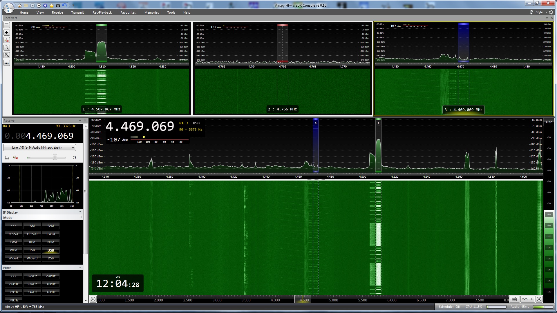
In early November, whilst working on an article for Janes, I noticed a Link-11 SLEW signal on 4510 kHz (CF) that was slowly growing in reception strength. I’d been monitoring frequencies used by the Northern Fleet of the Russian navy around this one and had already spotted that Link-11 CLEW was being used on a nearby frequency, though this remained at a constant signal strength at my location. The fact that the Link-11 SLEW was getting stronger made me stop what I was doing and start concentrating on this instead.
AirSpy HF+ Discovery SDR with SDRConsole operating software. Link-11 SLEW signal in Receiver 1, and the weaker Link-11 CLEW signal in Receiver 3. Whilst there a two SLEW signals showing, there is just one, with the left hand one being produced by the strong signal. You can see the weaker transmissions from a receiving station between the stronger ones on the correct frequency, but not on the “reflection”.
Link-11 SLEW (Single-Tone Link-11 waveform) ,or STANAG 5511, is a NATO Standard for tactical data exchange used between multiple platforms, be it on Land, Sea or Air. Its main function is the exchange of radar information, and in HF this is particularly useful for platforms that are beyond line of sight of each other and therefore cannot use the UHF version of Link-11.
With propagation being the way it is, in theory radar data could be exchanged between platforms that are hundreds to thousands of miles apart, therefore providing a wider picture of operations to other mobile platforms and fixed land bases. This data can also be forwarded on using ground stations that receive the data and then re-transmit on another frequency and/or frequency band. However, the approximate range of an individual broadcast on HF is reported to be 300nm.
As well as radar information, electronic warfare (EW) and command data can also be transmitted, but despite the capability to transmit radar data, it is not used for ATC purposes. In the UK, Link-11 is used by both the RAF (in E-3 AWAC’s and Tactical Air Control Centres) and the Royal Navy. Primarily it is used for sharing of Maritime data. Maritime Patrol Aircraft (MPA’s) such as USN P-8’s and Canadian CP-140’s use Link-11 both as receivers and transmitters of data, so when the RAF start using their P-8’s operationally in 2020 expect this to be added to the UK list. Whilst it is a secure data system, certain parameters can be extracted for network analysis and it can be subjected to Electronic Countermeasures (ECM).
Link-11 data is correlated against any tracks already present on a receivers radar picture. If a track is there it is ignored, whilst any that are missing are added but with a different symbol to show it is not being tracked by their own equipment. As this shared data is normally beyond the range of a ships own radar systems, this can provide an early warning of possible offensive aircraft, missiles or ships that would not normally be available.
I started up go2MONITOR and linked it to my WinRadio G31 Excalibur. Using a centre frequency of 4510 kHz I ran an emission search and selected the Link-11 SLEW modulation that it found at this frequency.
It immediately started decoding as much as it could, and I noticed that three Address ID’s were in the network.
go2MONITOR in action just after starting it up. Note, three ID’s in the network – 2_o, 30_o and 71_o
As the signal was strong, and it is normally maritime radar data that is being transmitted, I decided to have a quick look on AIS to see if there was anything showing nearby. Using AISLive I spotted that Norwegian navy Fridtjof Nansen class FFGHM Thor Heyerdahl was 18.5 nm SW of my location, just to the west of the island Ailsa Craig. Whilst it was using an incorrect name for AIS identification, its ITU callsign of LABH gave me the correct ID. This appeared to be the likely candidate for the strong Link-11 signal.
Position of Thor Heyerdahl from my AIS receiver using AISLive software
It wasn’t the best day and it was pretty murky out to sea with visibility being around 5nm – I certainly couldn’t see the Isle of Arran 11.5 nm away. I kept an eye on the AIS track for Thor Heyerdahl but it didn’t appear to be moving.
Whilst my own gear doesn’t allow me to carry out any Direction Finding (DF) I elected to utilise SDR.hu and KiwiSDR’s to see if I could get a good TDoA fix on a potential transmitter site – TDoA = Time Difference Of Arrival, also known as multilateration or MLAT. Whilst not 100% accurate, TDoA is surprisingly good and will sometimes get you to within a few kilometres of a transmission site with a strong signal.
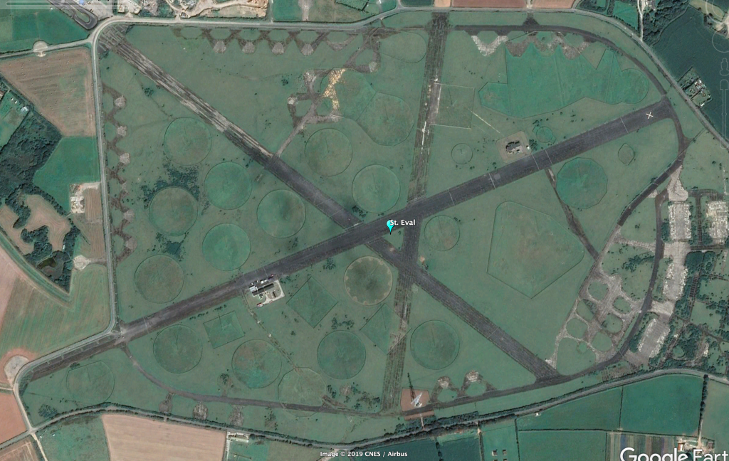
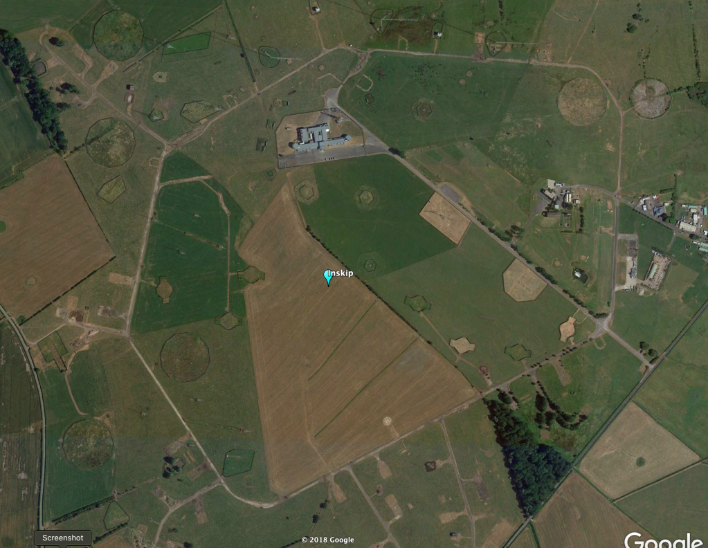
One of my thoughts was that the signal was emanating from the UK Defence High Frequency Communications Service (DHFCS) site at either St. Eval in Cornwall or Inskip in Lancashire. With this in mind I picked relevant KiwiSDR’s that surrounded these two sites and my area and ran a TDoA.
As expected, the result showed the probable transmitter site as just over 58 kilometres from St. Eval, though the overall shape and “hot area” of the TDoA map also covered Inskip, running along the West coast of England, Wales and Scotland. It peaked exactly in line to where the Norwegian navy ship and I were located! With the fact that there were signals being received from three different sources it is highly likely this has averaged out to this plot.
TDoA result showing the likely transmitter site at 50.60N 4.20W. Note the elongated “hot spot” which denotes the area that the transmitter site is likely to be situated.
Just after 10am the weather cleared allowing me to see a US Navy Arleigh Burke class DDGHM between myself and Arran. This added an extra ship to the equation, and also tied in with the TDoA hot spot. Things were getting even more interesting!
Link-11 SLEW at its strongest which also coincided with USS Gridley being its closest to my location.
Thor Heyerdahl still hadn’t moved according to AISLive but the Arleigh Burke was clearly heading in to the Royal Navy base at Faslane. With my Bearcat UBC-800T scanning the maritime frequencies it wasn’t long before “Warship 101” called up for Clyde pilot information along with an estimate for Ashton Buoy of 1300z. Warship 101 tied up with Arleigh Burke USS Gridley.
The Link-11 SLEW signal was considerably weaker at the time USS Gridley was at Ashton Buoy.
As USS Gridley progressed towards Faslane, the signal started to get weaker. Ashton Buoy is where most ships inbound for Faslane meet the pilot and tugs, taking up to another 30 minutes to get from there to alongside at the base – a journey of about 8.5nm.
At 1328z the Link-11 SLEW signal ended which coincided with the time that USS Gridley approached alongside at Faslane. It would be at about this time that most of the radar systems used on the ship would have been powered down so data was no longer available for transmission, therefore the Link-11 network was not required any further and it was disconnected.
Some images of USS Gridley arriving into Faslane taken by good friend Dougie Coull
So, was this Link-11 SLEW connected to USS Gridley? And was the ship also the NCS of the network? I think the answer is yes to both, and I’ll explain a couple of things that leads me to this conclusion. But first…………….
Link-11 SLEW Technical details
Using Upper Side Band (USB) in HF, a single waveform is generated in a PSK-8 modulated, 1800 Hz tone. The symbol rate is 2400 Bd and the user data rate is 1800 bps. Link-11 SLEW is an improved version of the older Link-11 CLEW modulation and due to enhanced error detection and correction is a more robust method of sending data. This makes it more likely that transmissions are received correctly the first time. Moreover, an adaptive system is used to counter any multipath signals the receiving unit may experience due to HF propagation.
The waveform transmission consists of an acquisition preamble followed by two or more fields, each of which is followed by a reinsertion probe. The field after the preamble is a header field containing information that is used by the CDS (Combat Data System) and an encryptor. If a network Participating Unit (PU) has any data, for instance track data, this follows the reinsertion probe. Finally, an end-of-message (EOM) is sent followed by a reinsertion probe.
The header is made up of 33 data bits and 12 error detection bits (CRC – Cyclic Redundancy Check). The 45 bit sequence is encoded with a 1/2 rate error correction code therefore giving a 90 bit field. The header contains information on the transmission type used, Picket/Participating Unit (PU) address, KG-40 Message Indicator, the NCS/Picket designation and a spare field.
Broken down, each piece of information is made up as follows:
The transmission type indicates the format of the transmission – 0 for a NCS (Network Control) Interrogation Message (NCS IM); 1 for a NCS Interrogation with Message (NCS IWM) or a Picket reply.
The address contains either the address of the next Picket or that of the Picket that initiated the call.
The KG-40 Message Indicator (MI) contains a number sequence generated by a KG-40AR cryptographic device. Synchronization is achieved when the receiver acquires the correct MI. For a NCS IM this will be made up of zeros as no message or data is actually sent.
The NCS/Picketdesignation identifies whether the current transmission originates from the NCS or PU: 0 = NCS; 1 = PU
Following on from the header, the SLEW data field consists of 48 information data bits along with 12 error detection and correction bits, themselves encoded with 2/3 rate error correction. This creates a 90 bit data field.
The EOM indicates the end of the transmission and is also a 90 bit field. There are no error detection or correction bits. Depending on the unit that is transmitting, a different sequence is sent – NCS = 0’s; PU = 1’s
Analysis
There is a specific order of transmissions which takes place for data to be exchanged.
Ordinarily the NCS sends data that creates the network, synchronizing things such as platform clocks etc. Each PU is called by the NCS and any data that a PU has is then sent, or the NCS sends data, or both. This is a very simple explanation of how data is exchanged but if you monitor a SLEW network you’ll see the exchanges take place rapidly. Except for the message itself which is encrypted, go2MONITOR will decode all the relevant information for you for analysis. This means that you don’t need to look at each raw data burst as sent to calculate whether it was a PU reply or NCS IWM, the decoder will do this for you.
At this point I need to say that Link-11 decoding is only available in the Mil version of go2MONITOR so doesn’t come as standard. Should you be interested in Link-11 decoding yourself then you would need to go for the full go2MONITOR package to enable this.
As previously mentioned, the data itself is encrypted but it is possible to try to calculate who is who within the network, and the analysis of the header information in particular will give you a good clue if you already know of potential PU’s that could be on the frequency.
In this case we already have four possible PU’s:
USS Gridley
Thor Heyerdahl
St. Eval transmitter site
Inskip transmitter site
It later transpired that Thor Heyerdahl had gone into Belfast Harbour for repairs so this practically cancelled out this ship as the NCS though it could still be a PU. Moreover, Thor Heyerdahl and USS Gridley were part of the same NATO squadron at that time which meant it was highly likely they were on the same network. This left us with three choices for the NCS, but still four for the network.
Here, I’d cancel out Inskip completely as both the NCS and a PU as the TDoA appeared to give a stronger indication to St. Eval – that left us with three in the network.
The pure fact that the strength of the major signal increased as USS Gridley got closer to my location, then slowly faded as she went further away added to my theory of her being the NCS. This was practically confirmed when the signal stopped on arrival to Faslane. Throughout the monitoring period he other signals on the frequency remained at the same strength.
Based on this, this meant that the strong signal was USS Gridley using ID Address 2_o.
Let’s take a look at one the previous screenshots, but this time with annotations explaining a number of points.
Firstly, we need to look for the NCS. The easiest way to do this is to look at the NCS/Picket Designation and find transmissions that are a zero, combined with a Message Type that indicates it is a NCS IWM. Here, there is just one transmission and that emanates from Address ID 2_o – the long one that includes a data message.
We next need to find NCS/Picket Designation transmissions that still have a zero – therefore coming from the NCS – but that have a Message Type that show it to be a NCS IM. These are calls from the NCS to any PU’s that are on the network looking to see if they have any “traffic” or messages.
Because of this there should be numerous messages of this type, and if you notice none have an ID address of 2_o. However, all of these messages are actually coming from 2_o as the ID address shown in a NCS IM is that of the PU being called rather than who it is from.
Any reply messages from PU’s will show as a NCS IWM/PU Reply transmission, but importantly the NCS/PU designation will be a one – showing it isn’t the NCS. Here there is one data reply from 71_o. You’ll notice that in the “reflection” there isn’t any transmission, unlike the ones from 2_o.
Moreover, though not shown here as the messages were off screen and not captured in the screen grab, you can see that one of the PU’s sent another reply message. As I was able to look at the complete message history I was able to see that this was also from 71_o – and 2_o either replied to this or sent further data.
There are two fainter transmissions which were not captured by go2MONITOR. These were from a PU, and must have been 30_o as there are no transmissions at all in the sequence that are from this ID address.
We now have a quandry. Who was 30_o and who was 71_o?
Data is definitely being sent by 71_o so to me this is more likely to be a ship rather than a transmitter site – but – a strong TDoA signal pointing at St. Eval makes it look like 71_o is this location instead.
Now though, we need to think outside the box a bit and realise that I’m looking at two different sources of radio reception. The TDoA receivers I selected were nowhere near my location as I’d selected KiwiSDR’s that surrounded St. Eval. This meant the signal that was weak with me could have been strong with these, therefore giving the result above.
If I base the fact that I think USS Gridley is 2_o due to strength, then I must presume the same with 71_o and call this as Thor Heyerdahl as this is the second strongest signal. I can also say that having gone through the four and a half hours of Link-11 SLEW transmissions available that 30_o never sent a single data transmission – or rather, not one that was received by me.
Full four and a half hours of Link-11 SLEW as shown in the go2MONITOR results page. You can see other areas (in red) that I was decoding at the same same. By selecting an area in the results page you can access the data as decoded, saved into files. I could have further enhanced this and carried out a full audio recording for further analysis, but I didn’t on this occasion.
Here then is my conclusion:
USS Gridley = 2_o and the NCS
Thor Heyerdahl = 71_o
St. Eval transmitter site = 30_o
Of course, we’ll never really know, but I hope this shows some of the extra things you can do with go2MONITOR and that it isn’t just a decoder. It really can add further interest to your radio monitoring if you’re an amateur; and if you’re a professional with a full plethora of gear, direction finders, receiver networks etc. then you really can start getting some interesting results in SIGINT gathering with this software – and highly likely be able to pinpoint exactly who was who in this scenario.
Now, how do I get some Direction Finders set up near me….Hmmmmmm??
The shack, finally operational after a few months off.
With the rebuild of my shack complete I’ve been able to start testing out all my radios, new connections etc.
The Mini-Circuits components all come well packaged in anti-static bags
A whole bundle of new cables from Mini-Circuits arrived last of all and have helped tidy up the back of the radio 19″ rack considerably. I’ve previously installed quite a few Mini-Circuits components, including 0.141″ diameter Hand-Flex interconnect cables, and so it was more of these that I opted for. The bonus with these cables is that they are hand formable meaning you can shape and bend them into pretty much any area that you want to. The 141 series (which I use) are capable of a 8mm bend radius, whilst the thinner 086 series can be bent to 6mm.
Being able to manipulate the cables certainly helps in tight spaces, and when you don’t want them to hang down
Previously I used hand-made cables with RG58U coax, but in order to have a 19″ rack that can slide out from under the desk, the cables needed to be longer than actually required. Because of this the cables would drop down into all the others attached to the PC and in some cases cause a little interference. With the Hand-Flex cables I’ve been able to use the same length of coax to allow me to move out the rack, but be able to bend them up and out of the way of the PC cables.
They’re also very good for the radios on the rack, being able to bend them and hold in place around the radios and other cables. They are near lossless too with a quoted insertion loss of 0.01 dB in the HF band to 0.55 dB at 18GHz. I normally run tests of the Mini-Circuit components when I receive them and find that the figures quoted are near spot on. I highly recommend these cables if you’re looking to upgrade your systems, and are available from the Mini-Circuits website, along with lots of other goodies that will tempt you.
Measurement of insertion loss of the Mini-Circuits ZF3RSC-542B-S+ Power Splitter/Combiner I also purchased as part of my plans for satellite communication monitoring. This is connected to the AirSpy SDR and takes feeds from two SatCom connections (currently deactivated) and a WinRadio AX-71C Discone Antenna. Mini-Circuits quote an insertion loss of around 19.5dB at 130 MHz which is confirmed here with a signal generated at -20dB being less than 1dB out at -40.48dB when passed through the combiner.
This image shows how the cables can be held in place without cable ties
The radio setup now includes two new SDR’s – an AirSpy HF+ and a standard AirSpy with the HF+ replacing the Enablia TitanPro. I’ve also reinstated my WinRadio G31DDC which had been in storage for a year or so. I really do like the TitanPro, and have put it into storage for the time being. The recording capabilities in particular are great with it being able to select 40 frequencies at once spread over numerous bandwidths, but I have had issues with the power supply – one being it caused interference. I attempted to make one of my own but it has a 6v(+/-1v)/2.5 Amp current requirement and no matter how many different methods of building my own supply using a 12v feed downgrading to 5, 6 or 7 volts, it just wouldn’t work in a stable manner. In the end it was easier to remove it and slot the G31DDC back in its place.
As it is, I’d forgotten how good the G31DDC is and I don’t really feel like I’m missing much thanks to the ability to use the other SDR’s with SDR Console V3 and it’s SDR Analyser.
The three 19″ racking units from Penn Elcom, along with all the shelves, have been very useful and certainly makes things easier when it comes to changing radios and connections over. I can just disconnect a few things and slide the whole unit out. I also obtained a 19″ Project box from them which I used as my main 12v switch unit. This is connected to two regulated desktop power supplies that act as master switches.
Although the SDR Console website page for the Analyser states it isn’t available yet, this is incorrect and it is downloaded with the latest version of the main programme.
If you’re a current user of V2 or have been in the past then you won’t notice much difference. You can have up to 24 parallel demodulators operating within the SDR’s bandwidth that you have chosen, all of which can run independent of each other in receive and record. You can also run each demodulator through a decoder such as MultiPSK independently and decode these in parallel with each other. This capability has taken that step towards those of the TitanPro, especially when being used with the Elad FDM-S2 that can provide a Maximum DDC bandwidth of 6144kHz’s.
Unfortunately, whilst you can schedule recordings of IQ data, you still can’t do this for individual channel recordings. This is a real shame as it would be a fantastic addition to the capabilities of SDR Console.
Getting back to the analyser though this does, in theory, cancel out the lack of channel recording scheduling.
When you record IQ data it is saved as WAV files, split into multiple ones depending on how long a recording you make . All of these files can be individually played back through the incorporated SDR Console player but even better is the use of the File Analyser.
With this you get a visual “image” of the complete recording, whereby after opening the analyser you get it to combine all the files into one XML file. For the image below I used the FDM-S2 with a selected bandwith of 768kHz centred on 4425kHz, hoping to catch calls to Russian Naval base Severomorsk in CW(RJD99) from ships operating in the region. I set the scheduler up to record from 0000z to 0700z which worked perfectly, giving me 78 files totalling 78GB – obviously, the bigger the bandwidth, the larger the total file size.
After clicking on New in the analyser and browsing to the relevant folder the WAV files are saved in, the analyser finds the first one and gives this as an option to open – it automatically adds the remaining WAV files and starts the process. This can take quite some time to extract, around 45 minutes for the example shown. But you only need to do this once because once it has finished you can save it as an XML file and open it at any time – in this case it was a 28MB XML file.
A note here – do not then delete the WAV files as the analyser still needs them.
As you can see, I was successful in locating calls to RJD99, and I have highlighted some of the others that I took a look at – this is just a screenshot of two hours out of the seven recorded.
All you then need to do is find any signal of interest, and after clicking on select and start in the top ribbon, click on the signal. This will then start playing the file from that location in the main SDR Console window. You don’t need to stay on that frequency, you can use the Console as if you were listening live and move around the frequency range you dictated in the bandwidth of the recording.
And, as it is basically a live screen you can do additional things such as record and use decoding software.
RJI92 calling RJD99 on 4416 kHz during playback of the Analyser
When using the Analyser I run this through a separate PC meaning SDR Console itself can carry on working on the main radio control PC. This is also handy if you’re away but have time to go through the IQ data using a laptop. Just copy over the original WAV files to a portable hard drive/memory stick and carry on as described above.
There are numerous other functions available for you to use with the main part of SDR Console, some I still haven’t had the chance to play with completely. I’m still exploring things such as the Signal History function which can store up to 48 hours of data. Here you can export data in CSV format to third-party programs such as QtiPlot. Signal history can also be used within the Analyser
This is useful as it can give you a quick overview into single frequency use, signal strengths, fading and such like. Definitely something I need to spend more time on.
It’s been a long time coming, but Version 3 of SDR Console has been well worth the wait.