
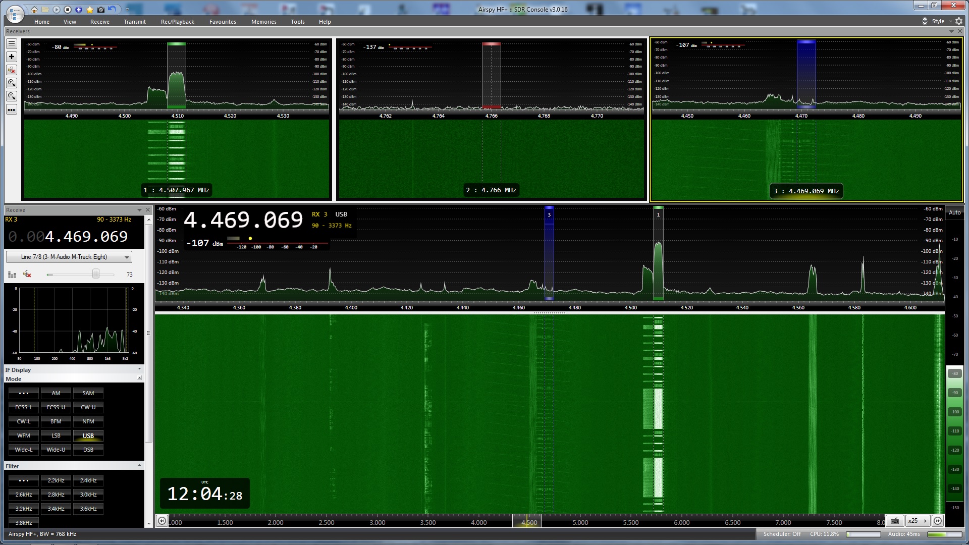
In early November, whilst working on an article for Janes, I noticed a Link-11 SLEW signal on 4510 kHz (CF) that was slowly growing in reception strength. I’d been monitoring frequencies used by the Northern Fleet of the Russian navy around this one and had already spotted that Link-11 CLEW was being used on a nearby frequency, though this remained at a constant signal strength at my location. The fact that the Link-11 SLEW was getting stronger made me stop what I was doing and start concentrating on this instead.
Link-11 SLEW (Single-Tone Link-11 waveform) ,or STANAG 5511, is a NATO Standard for tactical data exchange used between multiple platforms, be it on Land, Sea or Air. Its main function is the exchange of radar information, and in HF this is particularly useful for platforms that are beyond line of sight of each other and therefore cannot use the UHF version of Link-11.
With propagation being the way it is, in theory radar data could be exchanged between platforms that are hundreds to thousands of miles apart, therefore providing a wider picture of operations to other mobile platforms and fixed land bases. This data can also be forwarded on using ground stations that receive the data and then re-transmit on another frequency and/or frequency band. However, the approximate range of an individual broadcast on HF is reported to be 300nm.
As well as radar information, electronic warfare (EW) and command data can also be transmitted, but despite the capability to transmit radar data, it is not used for ATC purposes. In the UK, Link-11 is used by both the RAF (in E-3 AWAC’s and Tactical Air Control Centres) and the Royal Navy. Primarily it is used for sharing of Maritime data. Maritime Patrol Aircraft (MPA’s) such as USN P-8’s and Canadian CP-140’s use Link-11 both as receivers and transmitters of data, so when the RAF start using their P-8’s operationally in 2020 expect this to be added to the UK list. Whilst it is a secure data system, certain parameters can be extracted for network analysis and it can be subjected to Electronic Countermeasures (ECM).
Link-11 data is correlated against any tracks already present on a receivers radar picture. If a track is there it is ignored, whilst any that are missing are added but with a different symbol to show it is not being tracked by their own equipment. As this shared data is normally beyond the range of a ships own radar systems, this can provide an early warning of possible offensive aircraft, missiles or ships that would not normally be available.
I started up go2MONITOR and linked it to my WinRadio G31 Excalibur. Using a centre frequency of 4510 kHz I ran an emission search and selected the Link-11 SLEW modulation that it found at this frequency.
It immediately started decoding as much as it could, and I noticed that three Address ID’s were in the network.

As the signal was strong, and it is normally maritime radar data that is being transmitted, I decided to have a quick look on AIS to see if there was anything showing nearby. Using AISLive I spotted that Norwegian navy Fridtjof Nansen class FFGHM Thor Heyerdahl was 18.5 nm SW of my location, just to the west of the island Ailsa Craig. Whilst it was using an incorrect name for AIS identification, its ITU callsign of LABH gave me the correct ID. This appeared to be the likely candidate for the strong Link-11 signal.

It wasn’t the best day and it was pretty murky out to sea with visibility being around 5nm – I certainly couldn’t see the Isle of Arran 11.5 nm away. I kept an eye on the AIS track for Thor Heyerdahl but it didn’t appear to be moving.
Whilst my own gear doesn’t allow me to carry out any Direction Finding (DF) I elected to utilise SDR.hu and KiwiSDR’s to see if I could get a good TDoA fix on a potential transmitter site – TDoA = Time Difference Of Arrival, also known as multilateration or MLAT. Whilst not 100% accurate, TDoA is surprisingly good and will sometimes get you to within a few kilometres of a transmission site with a strong signal.
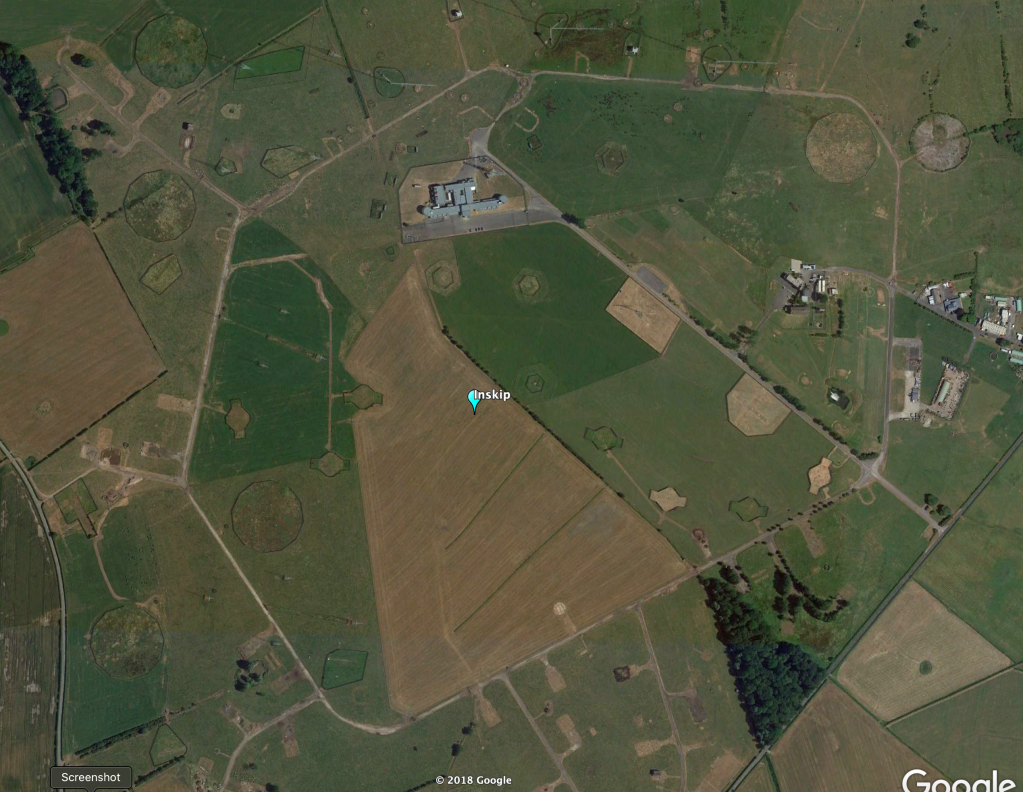
One of my thoughts was that the signal was emanating from the UK Defence High Frequency Communications Service (DHFCS) site at either St. Eval in Cornwall or Inskip in Lancashire. With this in mind I picked relevant KiwiSDR’s that surrounded these two sites and my area and ran a TDoA.
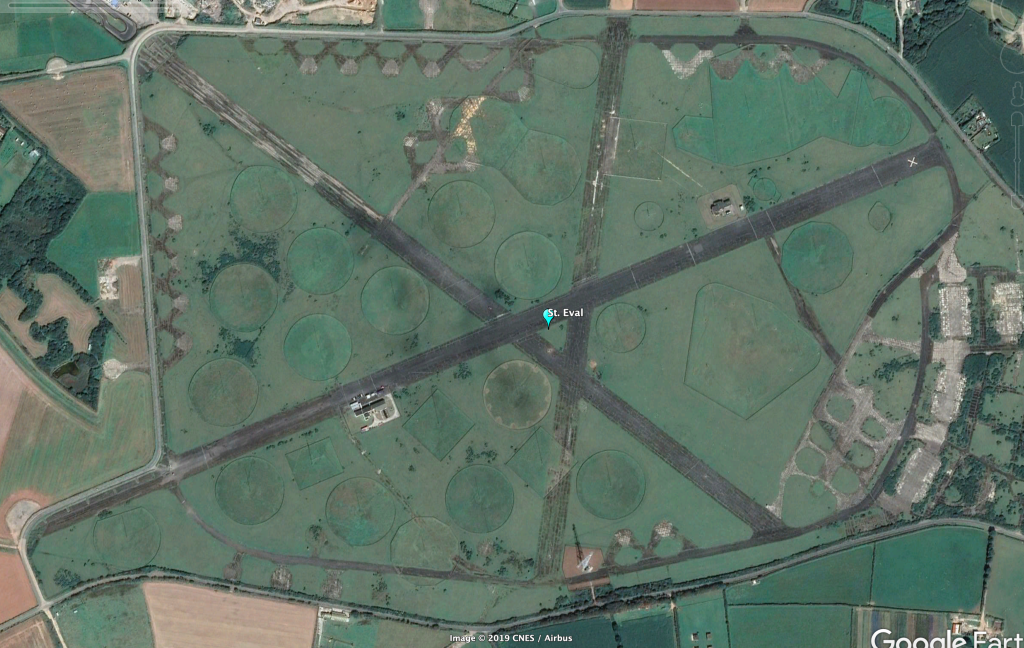
As expected, the result showed the probable transmitter site as just over 58 kilometres from St. Eval, though the overall shape and “hot area” of the TDoA map also covered Inskip, running along the West coast of England, Wales and Scotland. It peaked exactly in line to where the Norwegian navy ship and I were located! With the fact that there were signals being received from three different sources it is highly likely this has averaged out to this plot.


Just after 10am the weather cleared allowing me to see a US Navy Arleigh Burke class DDGHM between myself and Arran. This added an extra ship to the equation, and also tied in with the TDoA hot spot. Things were getting even more interesting!

Thor Heyerdahl still hadn’t moved according to AISLive but the Arleigh Burke was clearly heading in to the Royal Navy base at Faslane. With my Bearcat UBC-800T scanning the maritime frequencies it wasn’t long before “Warship 101” called up for Clyde pilot information along with an estimate for Ashton Buoy of 1300z. Warship 101 tied up with Arleigh Burke USS Gridley.

As USS Gridley progressed towards Faslane, the signal started to get weaker. Ashton Buoy is where most ships inbound for Faslane meet the pilot and tugs, taking up to another 30 minutes to get from there to alongside at the base – a journey of about 8.5nm.
At 1328z the Link-11 SLEW signal ended which coincided with the time that USS Gridley approached alongside at Faslane. It would be at about this time that most of the radar systems used on the ship would have been powered down so data was no longer available for transmission, therefore the Link-11 network was not required any further and it was disconnected.

So, was this Link-11 SLEW connected to USS Gridley? And was the ship also the NCS of the network? I think the answer is yes to both, and I’ll explain a couple of things that leads me to this conclusion. But first…………….
Link-11 SLEW Technical details
Using Upper Side Band (USB) in HF, a single waveform is generated in a PSK-8 modulated, 1800 Hz tone. The symbol rate is 2400 Bd and the user data rate is 1800 bps. Link-11 SLEW is an improved version of the older Link-11 CLEW modulation and due to enhanced error detection and correction is a more robust method of sending data. This makes it more likely that transmissions are received correctly the first time. Moreover, an adaptive system is used to counter any multipath signals the receiving unit may experience due to HF propagation.
The waveform transmission consists of an acquisition preamble followed by two or more fields, each of which is followed by a reinsertion probe. The field after the preamble is a header field containing information that is used by the CDS (Combat Data System) and an encryptor. If a network Participating Unit (PU) has any data, for instance track data, this follows the reinsertion probe. Finally, an end-of-message (EOM) is sent followed by a reinsertion probe.
The header is made up of 33 data bits and 12 error detection bits (CRC – Cyclic Redundancy Check). The 45 bit sequence is encoded with a 1/2 rate error correction code therefore giving a 90 bit field. The header contains information on the transmission type used, Picket/Participating Unit (PU) address, KG-40 Message Indicator, the NCS/Picket designation and a spare field.
Broken down, each piece of information is made up as follows:
The transmission type indicates the format of the transmission – 0 for a NCS (Network Control) Interrogation Message (NCS IM); 1 for a NCS Interrogation with Message (NCS IWM) or a Picket reply.
The address contains either the address of the next Picket or that of the Picket that initiated the call.
The KG-40 Message Indicator (MI) contains a number sequence generated by a KG-40AR cryptographic device. Synchronization is achieved when the receiver acquires the correct MI. For a NCS IM this will be made up of zeros as no message or data is actually sent.
The NCS/Picket designation identifies whether the current transmission originates from the NCS or PU: 0 = NCS; 1 = PU
Following on from the header, the SLEW data field consists of 48 information data bits along with 12 error detection and correction bits, themselves encoded with 2/3 rate error correction. This creates a 90 bit data field.
The EOM indicates the end of the transmission and is also a 90 bit field. There are no error detection or correction bits. Depending on the unit that is transmitting, a different sequence is sent – NCS = 0’s; PU = 1’s
Analysis
There is a specific order of transmissions which takes place for data to be exchanged.
Ordinarily the NCS sends data that creates the network, synchronizing things such as platform clocks etc. Each PU is called by the NCS and any data that a PU has is then sent, or the NCS sends data, or both. This is a very simple explanation of how data is exchanged but if you monitor a SLEW network you’ll see the exchanges take place rapidly. Except for the message itself which is encrypted, go2MONITOR will decode all the relevant information for you for analysis. This means that you don’t need to look at each raw data burst as sent to calculate whether it was a PU reply or NCS IWM, the decoder will do this for you.
At this point I need to say that Link-11 decoding is only available in the Mil version of go2MONITOR so doesn’t come as standard. Should you be interested in Link-11 decoding yourself then you would need to go for the full go2MONITOR package to enable this.
As previously mentioned, the data itself is encrypted but it is possible to try to calculate who is who within the network, and the analysis of the header information in particular will give you a good clue if you already know of potential PU’s that could be on the frequency.
In this case we already have four possible PU’s:
- USS Gridley
- Thor Heyerdahl
- St. Eval transmitter site
- Inskip transmitter site
It later transpired that Thor Heyerdahl had gone into Belfast Harbour for repairs so this practically cancelled out this ship as the NCS though it could still be a PU. Moreover, Thor Heyerdahl and USS Gridley were part of the same NATO squadron at that time which meant it was highly likely they were on the same network. This left us with three choices for the NCS, but still four for the network.
Here, I’d cancel out Inskip completely as both the NCS and a PU as the TDoA appeared to give a stronger indication to St. Eval – that left us with three in the network.
The pure fact that the strength of the major signal increased as USS Gridley got closer to my location, then slowly faded as she went further away added to my theory of her being the NCS. This was practically confirmed when the signal stopped on arrival to Faslane. Throughout the monitoring period he other signals on the frequency remained at the same strength.
Based on this, this meant that the strong signal was USS Gridley using ID Address 2_o.
Let’s take a look at one the previous screenshots, but this time with annotations explaining a number of points.

Firstly, we need to look for the NCS. The easiest way to do this is to look at the NCS/Picket Designation and find transmissions that are a zero, combined with a Message Type that indicates it is a NCS IWM. Here, there is just one transmission and that emanates from Address ID 2_o – the long one that includes a data message.
We next need to find NCS/Picket Designation transmissions that still have a zero – therefore coming from the NCS – but that have a Message Type that show it to be a NCS IM. These are calls from the NCS to any PU’s that are on the network looking to see if they have any “traffic” or messages.
Because of this there should be numerous messages of this type, and if you notice none have an ID address of 2_o. However, all of these messages are actually coming from 2_o as the ID address shown in a NCS IM is that of the PU being called rather than who it is from.
Any reply messages from PU’s will show as a NCS IWM/PU Reply transmission, but importantly the NCS/PU designation will be a one – showing it isn’t the NCS. Here there is one data reply from 71_o. You’ll notice that in the “reflection” there isn’t any transmission, unlike the ones from 2_o.
Moreover, though not shown here as the messages were off screen and not captured in the screen grab, you can see that one of the PU’s sent another reply message. As I was able to look at the complete message history I was able to see that this was also from 71_o – and 2_o either replied to this or sent further data.
There are two fainter transmissions which were not captured by go2MONITOR. These were from a PU, and must have been 30_o as there are no transmissions at all in the sequence that are from this ID address.
We now have a quandry. Who was 30_o and who was 71_o?
Data is definitely being sent by 71_o so to me this is more likely to be a ship rather than a transmitter site – but – a strong TDoA signal pointing at St. Eval makes it look like 71_o is this location instead.
Now though, we need to think outside the box a bit and realise that I’m looking at two different sources of radio reception. The TDoA receivers I selected were nowhere near my location as I’d selected KiwiSDR’s that surrounded St. Eval. This meant the signal that was weak with me could have been strong with these, therefore giving the result above.
If I base the fact that I think USS Gridley is 2_o due to strength, then I must presume the same with 71_o and call this as Thor Heyerdahl as this is the second strongest signal. I can also say that having gone through the four and a half hours of Link-11 SLEW transmissions available that 30_o never sent a single data transmission – or rather, not one that was received by me.

Here then is my conclusion:
- USS Gridley = 2_o and the NCS
- Thor Heyerdahl = 71_o
- St. Eval transmitter site = 30_o
Of course, we’ll never really know, but I hope this shows some of the extra things you can do with go2MONITOR and that it isn’t just a decoder. It really can add further interest to your radio monitoring if you’re an amateur; and if you’re a professional with a full plethora of gear, direction finders, receiver networks etc. then you really can start getting some interesting results in SIGINT gathering with this software – and highly likely be able to pinpoint exactly who was who in this scenario.
Now, how do I get some Direction Finders set up near me….Hmmmmmm??


